
Concept explainers
Videos
Construct the ANOVA table and test for significance at 5% level.
Answer to Problem 58SE
The ANOVA table is given below:
| Source |
Degrees of freedom |
Sum of squares |
Mean sum of squares | F-ratio |
|
Vat pressure A | 1 | 6.94 | 6.94 | 11.57 |
|
Cooking time B | 3 | 5.61 | 1.87 | 3.12 |
|
Concentration C | 2 | 12.33 | 6.165 | 10.28 |
| Interaction AB | 3 | 4.05 | 1.35 | 2.25 |
| Interaction BC | 6 | 15.80 | 2.63 | 4.38 |
| Interaction AC | 2 | 7.32 | 3.66 | 6.10 |
| Interaction ABC | 6 | 4.37 | 0.728 | 1.21 |
| Error | 24 | 14.40 | 0.6 | |
| Total | 47 | 70.82 |
There is sufficient of evidence to conclude that there is an effect of vat pressure on the strength of the paper at 5% level of significance.
There is sufficient of evidence to conclude that there is an effect of cooking times on the strength of the paper at 5% level of significance.
There is sufficient of evidence to conclude that there is an effect of concentrations on the strength of the paper at 5% level of significance.
There is no sufficient of evidence to conclude that there is an interaction effect of vat pressure and cooking times on the strength of the paper at 5% level of significance.
There is sufficient of evidence to conclude that there is an interaction effect of cooking times and concentrations on the strength of the paper at 5% level of significance.
There is sufficient of evidence to conclude that there is an interaction effect of vat pressure and concentrations on the strength of the paper at 5% level of significance.
There is no sufficient of evidence to conclude that there is an interaction effect of vat pressure and concentrations on the strength of the paper at 5% level of significance.
Explanation of Solution
Given info:
An experiment was carried out to test the vat pressure A, cooking time of pulp B and hardwood concentration C on the strength of the paper.
The sum of squares of factor A is 6.94, due to factor B is 5.61, due to factor C is 12.33, due to interaction AB is 4.05, due to interaction BC is 15.80, due to interaction AC is 7.32, sum of squares due to error and total sum of squares is 14.40 and 70.82.
Two observations were made at each combination of factor levels.
Calculation:
The sum of squares due to the interaction of factor A, B and C is calculated as follows:
The general ANOVA table is given below:
| Source | Degrees of freedom | Sum of squares | Mean sum of squares | F-ratio |
| Factor A | ||||
| Factor B | ||||
| Factor C | ||||
| Interaction AB | ||||
| Error | ||||
| Total |
The ANOVA for the given data is shown below:
| Source | Degrees of freedom |
Sum of squares | Mean sum of squares | F-ratio |
|
Vat pressure A | 6.94 | 11.57 | ||
|
Cooking time B | 5.61 | 3.12 | ||
|
Concentration C | 12.33 | 10.28 | ||
| Interaction AB | 4.05 | 2.25 | ||
| Interaction BC | 15.80 | 4.38 | ||
| Interaction AC | 7.32 | 6.10 | ||
| Interaction ABC | 4.37 | 1.21 | ||
| Error | 14.40 | |||
| Total | 70.82 |
Where, the F statistic for each factor is obtained by dividing the mean sum of squares with the mean error sum of squares (MSE).
Testing the Hypothesis for the main effect A:
Null hypothesis:
That is, there is no significant difference in the strength of the paper due to the two levels of vat pressure.
Alternative hypothesis:
That is, there is significant difference in the strength of the paper due to the two levels of vat pressure.
Testing the Hypothesis for the main effect B:
Null hypothesis:
That is, there is no significant difference in the strength of the paper due to the four levels of cooking times.
Alternative hypothesis:
That is, there is significant difference in the strength of the paper due to the four levels of cooking times.
Testing the Hypothesis for the main effect C:
Null hypothesis:
That is, there is no significant difference in the strength of the paper due to the three levels of concentrations.
Alternative hypothesis:
That is, there is a significant difference in the strength of the paper due to the three levels of concentrations.
Testing the Hypothesis for the interaction effect of AB:
Null hypothesis:
That is, there is no significant difference in the strength due to the interaction between vat pressure and cooking times.
Alternative hypothesis:
That is, there is significant difference in the strength due to the interaction between vat pressure and cooking times.
Testing the Hypothesis for the interaction effect BC:
Null hypothesis:
That is, there is no significant difference in the strength due to the interaction between cooking times and concentrations.
Alternative hypothesis:
That is, there is significant difference in the strength due to the interaction between cooking times and concentrations.
Testing the Hypothesis for the interaction effect AC:
Null hypothesis:
That is, there is no significant difference in the strength of the paper due to the interaction between vat pressure and concentrations.
Alternative hypothesis:
That is, there is a significant difference in the strength of the paper due to the interaction between vat pressure and concentrations.
Testing the Hypothesis for the interaction effect ABC:
Null hypothesis:
That is, there is no significant difference in the strength of the paper due to the interaction between vat pressure, cooking times and concentrations.
Alternative hypothesis:
That is, there is a significant difference in the strength of the paper due to the interaction between vat pressure, cooking times and concentrations.
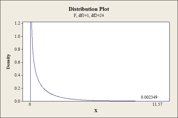
P-value for the main effect of A:
Software procedure:
Step-by-step procedure to find the P-value is given below:
- Click on Graph, select View Probability and click OK.
- Select F, enter 1 in numerator df and 24 in denominator df.
- Under Shaded Area Tab select X value under Define Shaded Area By and select right tail.
- Choose X value as 11.57.
- Click OK.
Output obtained from MINITAB is given below:
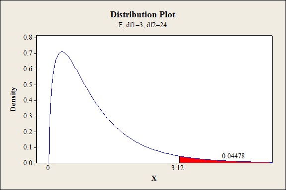
P-value for the main effect of B:
Software procedure:
Step-by-step procedure to find the P-value is given below:
- Click on Graph, select View Probability and click OK.
- Select F, enter 3 in numerator df and 24 in denominator df.
- Under Shaded Area Tab select X value under Define Shaded Area By and select right tail.
- Choose X value as 3.12.
- Click OK.
Output obtained from MINITAB is given below:
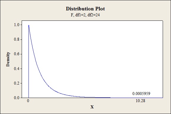
P-value for the main effect of C:
Software procedure:
Step-by-step procedure to find the P-value is given below:
- Click on Graph, select View Probability and click OK.
- Select F, enter 2 in numerator df and 24 in denominator df.
- Under Shaded Area Tab select X value under Define Shaded Area By and select right tail.
- Choose X value as 10.28.
- Click OK.
Output obtained from MINITAB is given below:
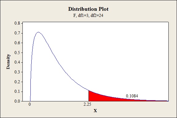
P-value for the interaction effect of AB:
Software procedure:
Step-by-step procedure to find the P-value is given below:
- Click on Graph, select View Probability and click OK.
- Select F, enter 3 in numerator df and 24 in denominator df.
- Under Shaded Area Tab select X value under Define Shaded Area By and select right tail.
- Choose X value as 2.25.
- Click OK.
Output obtained from MINITAB is given below:
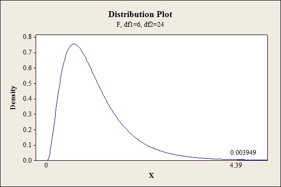
P-value for the interaction effect of BC:
Software procedure:
Step-by-step procedure to find the P-value is given below:
- Click on Graph, select View Probability and click OK.
- Select F, enter 6 in numerator df and 24 in denominator df.
- Under Shaded Area Tab select X value under Define Shaded Area By and select right tail.
- Choose X value as 4.39.
- Click OK.
Output obtained from MINITAB is given below:
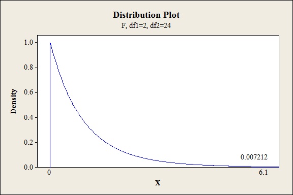
P-value for the interaction effect of AC:
Software procedure:
Step-by-step procedure to find the P-value is given below:
- Click on Graph, select View Probability and click OK.
- Select F, enter 2 in numerator df and 24 in denominator df.
- Under Shaded Area Tab select X value under Define Shaded Area By and select right tail.
- Choose X value as 6.10.
- Click OK.
Output obtained from MINITAB is given below:
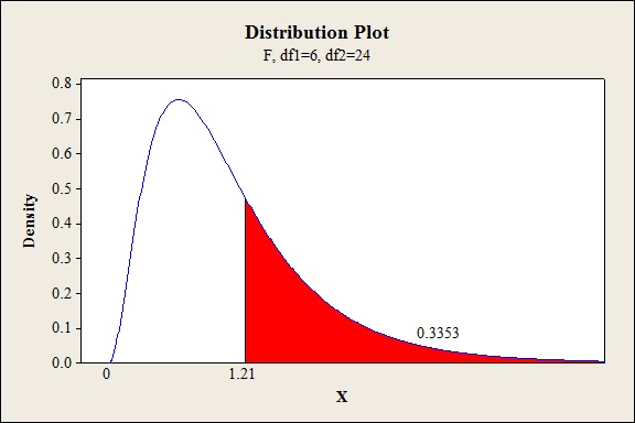
P-value for the interaction effect of ABC:
Software procedure:
Step-by-step procedure to find the P-value is given below:
- Click on Graph, select View Probability and click OK.
- Select F, enter 6 in numerator df and 24 in denominator df.
- Under Shaded Area Tab select X value under Define Shaded Area By and select right tail.
- Choose X value as 1.21.
- Click OK.
Output obtained from MINITAB is given below:
Conclusion:
For the main effect of A:
The P- value for the factor A (vat pressure) is 0.002 and the level of significance is 0.05.
Here, the P- value is lesser than the level of significance.
That is,
Thus, the null hypothesis is rejected,
Hence, there is sufficient of evidence to conclude that there is an effect of vat pressure on the strength of the paper at 5% level of significance.
For main effect of B:
The P- value for the factor B (cooking times) is 0.044 and the level of significance is 0.05.
Here, the P- value is lesser than the level of significance.
That is,
Thus, the null hypothesis is rejected.
Hence, there is sufficient of evidence to conclude that there is an effect of cooking times on the strength of the paper at 5% level of significance.
For main effect of C:
The P- value for the factor C (concentrations) is 0.000 and the level of significance is 0.05.
Here, the P- value is lesser than the level of significance.
That is,
Thus, the null hypothesis is rejected.
Hence, there is sufficient of evidence to conclude that there is an effect of concentrations on the strength of the paper at 5% level of significance.
For the interaction effect of AB:
The P- value for the interaction effect AB (vat pressure and cooking times) is 0.1084 and the level of significance is 0.05.
Here, the P- value is greater than the level of significance.
That is,
Thus, the null hypothesis is not rejected,
Hence, there is no sufficient of evidence to conclude that there is an interaction effect of vat pressure and cooking times on the strength of the paper at 5% level of significance.
For the interaction effect of BC
The P- value for the interaction effect BC (cooking times and concentrations) is 0.004 and the level of significance is 0.05.
Here, the P- value is lesser than the level of significance.
That is,
Thus, the null hypothesis is rejected,
Hence, there is sufficient of evidence to conclude that there is an interaction effect of cooking times and concentrations on the strength of the paper at 5% level of significance.
For the interaction effect of AC:
The P- value for the interaction effect AC (vat pressure and concentrations) is 0.0072 and the level of significance is 0.05.
Here, the P- value is lesser than the level of significance.
That is,
Thus, the null hypothesis is rejected,
Hence, there is sufficient of evidence to conclude that there is an interaction effect of vat pressure and concentrations on the strength of the paper at 5% level of significance.
For the interaction effect of ABC:
The P- value for the interaction effect ABC (vat pressure, cooking times and concentrations) is 0.3353 and the level of significance is 0.05.
Here, the P- value is greater than the level of significance.
That is,
Thus, the null hypothesis is not rejected,
Hence, there is no sufficient of evidence to conclude that there is an interaction effect of vat pressure, cooking times and concentrations on the strength of the paper at 5% level of significance.
The main effect A, B and C appears to be significant at 5% level. The interactions BC and AC are significant at 5% level of significance and the interactions AB and ABC are not significant at 5% level of significance.
Want to see more full solutions like this?
Chapter 11 Solutions
Student Solutions Manual for Devore's Probability and Statistics for Engineering and the Sciences, 9th


- Table of hours of television watched per week: 11 15 24 34 36 22 20 30 12 32 24 36 42 36 42 26 37 39 48 35 26 29 27 81276 40 54 47 KARKE 31 35 42 75 35 46 36 42 65 28 54 65 28 23 28 23669 34 43 35 36 16 19 19 28212 Using the data above, construct a frequency table according the following classes: Number of Hours Frequency Relative Frequency 10-19 20-29 |30-39 40-49 50-59 60-69 70-79 80-89 From the frequency table above, find a) the lower class limits b) the upper class limits c) the class width d) the class boundaries Statistics 300 Frequency Tables and Pictures of Data, page 2 Using your frequency table, construct a frequency and a relative frequency histogram labeling both axes.arrow_forwardA study was undertaken to compare respiratory responses of hypnotized and unhypnotized subjects. The following data represent total ventilation measured in liters of air per minute per square meter of body area for two independent (and randomly chosen) samples. Analyze these data using the appropriate non-parametric hypothesis test. Unhypnotized: 5.0 5.3 5.3 5.4 5.9 6.2 6.6 6.7 Hypnotized: 5.8 5.9 6.2 6.6 6.7 6.1 7.3 7.4arrow_forwardThe class will include a data exercise where students will be introduced to publicly available data sources. Students will gain experience in manipulating data from the web and applying it to understanding the economic and demographic conditions of regions in the U.S. Regions and topics of focus will be determined (by the student with instructor approval) prior to April. What data exercise can I do to fulfill this requirement? Please explain.arrow_forward
- Consider the ceocomp dataset of compensation information for the CEO’s of 100 U.S. companies. We wish to fit aregression model to assess the relationship between CEO compensation in thousands of dollars (includes salary andbonus, but not stock gains) and the following variates:AGE: The CEOs age, in yearsEDUCATN: The CEO’s education level (1 = no college degree; 2 = college/undergrad. degree; 3 = grad. degree)BACKGRD: Background type(1= banking/financial; 2 = sales/marketing; 3 = technical; 4 = legal; 5 = other)TENURE: Number of years employed by the firmEXPER: Number of years as the firm CEOSALES: Sales revenues, in millions of dollarsVAL: Market value of the CEO's stock, in natural logarithm unitsPCNTOWN: Percentage of firm's market value owned by the CEOPROF: Profits of the firm, before taxes, in millions of dollars1) Create a scatterplot matrix for this dataset. Briefly comment on the observed relationships between compensationand the other variates.Note that companies with negative…arrow_forward6 (Model Selection, Estimation and Prediction of GARCH) Consider the daily returns rt of General Electric Company stock (ticker: "GE") from "2021-01-01" to "2024-03-31", comprising a total of 813 daily returns. Using the "fGarch" package of R, outputs of fitting three GARCH models to the returns are given at the end of this question. Model 1 ARCH (1) with standard normal innovations; Model 2 Model 3 GARCH (1, 1) with Student-t innovations; GARCH (2, 2) with Student-t innovations; Based on the outputs, answer the following questions. (a) What can be inferred from the Standardized Residual Tests conducted on Model 1? (b) Which model do you recommend for prediction between Model 2 and Model 3? Why? (c) Write down the fitted model for the model that you recommended in Part (b). (d) Using the model recommended in Part (b), predict the conditional volatility in the next trading day, specifically trading day 814.arrow_forward4 (MLE of ARCH) Suppose rt follows ARCH(2) with E(rt) = 0, rt = ut, ut = στει, σε where {+} is a sequence of independent and identically distributed (iid) standard normal random variables. With observations r₁,...,, write down the log-likelihood function for the model esti- mation.arrow_forward
- 5 (Moments of GARCH) For the GARCH(2,2) model rt = 0.2+0.25u1+0.05u-2 +0.30% / -1 +0.20% -2, find cov(rt). 0.0035 ut, ut = στει,στ =arrow_forwardDefinition of null hypothesis from the textbook Definition of alternative hypothesis from the textbook Imagine this: you suspect your beloved Chicken McNugget is shrinking. Inflation is hitting everything else, so why not the humble nugget too, right? But your sibling thinks you’re just being dramatic—maybe you’re just extra hungry today. Determined to prove them wrong, you take matters (and nuggets) into your own hands. You march into McDonald’s, get two 20-piece boxes, and head home like a scientist on a mission. Now, before you start weighing each nugget like they’re precious gold nuggets, let’s talk hypotheses. The average weight of nuggets as mentioned on the box is 16 g each. Develop your null and alternative hypotheses separately. Next, you weigh each nugget with the precision of a jeweler and find they average out to 15.5 grams. You also conduct a statistical analysis, and the p-value turns out to be 0.01. Based on this information, answer the following questions. (Remember,…arrow_forwardBusiness Discussarrow_forward
- Cape Fear Community Colle X ALEKS ALEKS - Dorothy Smith - Sec X www-awu.aleks.com/alekscgi/x/Isl.exe/10_u-IgNslkr7j8P3jH-IQ1w4xc5zw7yX8A9Q43nt5P1XWJWARE... Section 7.1,7.2,7.3 HW 三 Question 21 of 28 (1 point) | Question Attempt: 5 of Unlimited The proportion of phones that have more than 47 apps is 0.8783 Part: 1 / 2 Part 2 of 2 (b) Find the 70th The 70th percentile of the number of apps. Round the answer to two decimal places. percentile of the number of apps is Try again Skip Part Recheck Save 2025 Mcarrow_forwardHi, I need to sort out where I went wrong. So, please us the data attached and run four separate regressions, each using the Recruiters rating as the dependent variable and GMAT, Accept Rate, Salary, and Enrollment, respectively, as a single independent variable. Interpret this equation. Round your answers to four decimal places, if necessary. If your answer is negative number, enter "minus" sign. Equation for GMAT: Ŷ = _______ + _______ GMAT Equation for Accept Rate: Ŷ = _______ + _______ Accept Rate Equation for Salary: Ŷ = _______ + _______ Salary Equation for Enrollment: Ŷ = _______ + _______ Enrollmentarrow_forwardQuestion 21 of 28 (1 point) | Question Attempt: 5 of Unlimited Dorothy ✔ ✓ 12 ✓ 13 ✓ 14 ✓ 15 ✓ 16 ✓ 17 ✓ 18 ✓ 19 ✓ 20 = 21 22 > How many apps? According to a website, the mean number of apps on a smartphone in the United States is 82. Assume the number of apps is normally distributed with mean 82 and standard deviation 30. Part 1 of 2 (a) What proportion of phones have more than 47 apps? Round the answer to four decimal places. The proportion of phones that have more than 47 apps is 0.8783 Part: 1/2 Try again kip Part ی E Recheck == == @ W D 80 F3 151 E R C レ Q FA 975 % T B F5 10 の 000 园 Save For Later Submit Assignment © 2025 McGraw Hill LLC. All Rights Reserved. Terms of Use | Privacy Center | Accessibility Y V& U H J N * 8 M I K O V F10 P = F11 F12 . darrow_forward
 College Algebra (MindTap Course List)AlgebraISBN:9781305652231Author:R. David Gustafson, Jeff HughesPublisher:Cengage Learning
 Algebra: Structure And Method, Book 1AlgebraISBN:9780395977224Author:Richard G. Brown, Mary P. Dolciani, Robert H. Sorgenfrey, William L. ColePublisher:McDougal Littell
 Glencoe Algebra 1, Student Edition, 9780079039897...AlgebraISBN:9780079039897Author:CarterPublisher:McGraw Hill
 Holt Mcdougal Larson Pre-algebra: Student Edition...AlgebraISBN:9780547587776Author:HOLT MCDOUGALPublisher:HOLT MCDOUGAL
 Linear Algebra: A Modern IntroductionAlgebraISBN:9781285463247Author:David PoolePublisher:Cengage Learning
 College AlgebraAlgebraISBN:9781305115545Author:James Stewart, Lothar Redlin, Saleem WatsonPublisher:Cengage Learning