
Videos
The accompanying data resulted from an experiment to investigate whether yield from a certain chemical process depended either on the formulation of a particular input or on mixer speed.
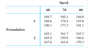
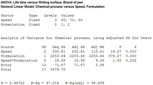
A statistical computer package gave SS(Form) = 2253.44, SS(Speed) = 230.81, SS(Form*Speed) = 18.58, and SSE = 71.87.
a. Does there appear to be interaction between the factors?
b. Does yield appear to depend on either formulation or speed?
c. Calculate estimates of the main effects.
d. The fitted values are
e. Construct a normal
a.
Identify whether there is a significant effect from interaction between speed and formulation.
Answer to Problem 18E
There is no sufficient evidence to conclude that there is an effect of interaction between mix speed and formulation on the chemical process.
Explanation of Solution
Given info:
An experiment was carried out to test the effect of formulation and speed on the chemical press. The formulation has two levels and speed has three levels.
The sum of squares due to formulation is 2,253.44, sum of squares due to speed is 230.81, sum of squares due to error is 71.87, sum of squares due to interaction between formulation and speed is 18.58.
Calculation:
Testing the Hypothesis:
Null hypothesis:
That is, the interaction effect between mix speed and formulation has no significant effect on chemical process.
Alternative hypothesis:
That is, the interaction effect between mix speed and formulation has no significant effect on chemical process.
Test statistic:
Software procedure:
Step by step procedure to find the test statistic using Minitab is given below:
- Choose Stat > ANOVA > General Linear Model.
- In Responses, enter the column of Chemical process.
- In Model, enter the column of Speed, Formulation, Speed*Formulation.
- In Results, choose “Analysis of variance table”.
- Click OK in all dialog boxes.
Output obtained from MINITAB is given below:
Conclusion:
Interaction effect of AB:
The P- value for the interaction effect AB is 0.252 and the level of significance is 0.01.
The P- value is lesser than the level of significance.
That is,
Thus, the null hypothesis is not rejected,
Hence, there is no sufficient evidence to conclude that there is an effect of interaction between mix speed and formulation on the chemical process.
b.
Identify whether the yield of the chemical process depends on speed or formulation.
Answer to Problem 18E
The yield of a chemical process depends on both speed and formulation.
Explanation of Solution
From the MINITAB output obtained in part (a), the following can be observed.
For Main effect of factor A speed:
The P- value for the factor A (speed) is 0.000 and the level of significance is 0.01.
The P- value is lesser than the level of significance.
That is,.
Thus, the null hypothesis is rejected,
Hence, there is sufficient evidence to conclude that there is an effect of speed on the yield of chemical process.
For Main effect of factor B formulation:
The P- value for the factor B (formulation) is 0.000 and the level of significance is 0.01.
The P- value is lesser than the level of significance.
That is,
Thus, the null hypothesis is rejected,
Hence, there is sufficient evidence to conclude that there is an effect of formulation on the yield of chemical process.
c.
Find the estimates for the main effects.
Explanation of Solution
Calculation:
Where,
Overall mean effect:
Mean due to the first level of factor A:
Mean due to the second level of factor A:
Main effect of factor A:
At first level:
At second level:
Mean due to the first level of factor B:
Mean due to the second level of factor B:
Mean due to the third level of factor B
Main effect of factor B:
d.
Verify whether the calculated residuals are equal to the given residual values.
Explanation of Solution
Calculation:
The interaction effect for the first level of factor A and the first level of factor B
The interaction effect for the first level of factor A and the second level of factor B
The interaction effect for the first level of factor A and the third level of factor B
Similarly, the remaining values are given below:
| S. No | Values |
| 1 | |
| 2 | |
| 3 | |
| 4 | |
| 5 | |
| 6 |
The fitted values are calculated by using the formula:
Where,
i represents the levels of factor A.
j represents the levels of factor B.
k represents the observation.
The predicted value when
Similarly, the other fitted values are calculated, the table shows the fitted values:
| S. No | 1 | 2 | 3 | 4 | 5 | 6 | 7 | 8 | 9 |
| Fitted values | 189.47 | 189.47 | 189.47 | 166.20 | 166.20 | 166.20 | 180.60 | 180.60 | 180.60 |
| S. No | 10 | 11 | 12 | 13 | 14 | 15 | 16 | 17 | 18 |
| Fitted values | 161.03 | 161.03 | 161.03 | 191.03 | 191.03 | 191.03 | 166.73 | 166.73 | 166.73 |
The residuals values are calculated by using the formula:
The table shows below gives the residuals for each observation:
| S. No |
Observed |
Fitted values | |
| 1 | 189.7 | 189.47 | 0.23 |
| 2 | 188.6 | 189.47 | –0.87 |
| 3 | 190.1 | 189.47 | 0.63 |
| 4 | 165.1 | 166.20 | –1.1 |
| 5 | 165.9 | 166.20 | –0.3 |
| 6 | 167.6 | 166.20 | 1.4 |
| 7 | 185.1 | 180.60 | 4.5 |
| 8 | 179.4 | 180.60 | –1.2 |
| 9 | 177.3 | 180.60 | –3.3 |
| 10 | 161.7 | 161.03 | 0.67 |
| 11 | 159.8 | 161.03 | –1.23 |
| 12 | 161.6 | 161.03 | 0.57 |
| 13 | 189 | 191.03 | –2.03 |
| 14 | 193 | 191.03 | 1.97 |
| 15 | 191.1 | 191.03 | 0.07 |
| 16 | 163.3 | 166.73 | –3.43 |
| 17 | 166.6 | 166.73 | –0.13 |
| 18 | 170.3 | 166.73 | 3.57 |
Hence, the calculated residuals values are equal to given residual values.
e.
Construct a normal probability plot for the residuals obtained in part (d).
Identify whether the residuals are normally distributed.
Answer to Problem 18E
The normal probability of residuals is given below:
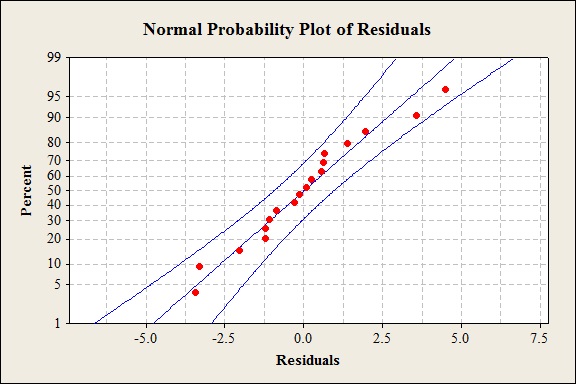
The residuals are normally distributed.
Explanation of Solution
Calculation:
Normal probability plot of residuals:
Software procedure:
Step-by-step procedure to construct a normal probability plot of residuals is given below:
- Click on Graph>Probability plot>Single.
- Click OK.
- Under Graph variables, select the column containing the residual values.
- Click on Distribution and selection Normal.
- Click OK.
Interpretation:
The normal probability plot of residuals suggests that the residuals are normally distributed because the residuals fall approximately on a straight line.
Want to see more full solutions like this?
Chapter 11 Solutions
Probability and Statistics for Engineering and the Sciences


- Examine the Variables: Carefully review and note the names of all variables in the dataset. Examples of these variables include: Mileage (mpg) Number of Cylinders (cyl) Displacement (disp) Horsepower (hp) Research: Google to understand these variables. Statistical Analysis: Select mpg variable, and perform the following statistical tests. Once you are done with these tests using mpg variable, repeat the same with hp Mean Median First Quartile (Q1) Second Quartile (Q2) Third Quartile (Q3) Fourth Quartile (Q4) 10th Percentile 70th Percentile Skewness Kurtosis Document Your Results: In RStudio: Before running each statistical test, provide a heading in the format shown at the bottom. “# Mean of mileage – Your name’s command” In Microsoft Word: Once you've completed all tests, take a screenshot of your results in RStudio and paste it into a Microsoft Word document. Make sure that snapshots are very clear. You will need multiple snapshots. Also transfer these results to the…arrow_forward2 (VaR and ES) Suppose X1 are independent. Prove that ~ Unif[-0.5, 0.5] and X2 VaRa (X1X2) < VaRa(X1) + VaRa (X2). ~ Unif[-0.5, 0.5]arrow_forward8 (Correlation and Diversification) Assume we have two stocks, A and B, show that a particular combination of the two stocks produce a risk-free portfolio when the correlation between the return of A and B is -1.arrow_forward
- 9 (Portfolio allocation) Suppose R₁ and R2 are returns of 2 assets and with expected return and variance respectively r₁ and 72 and variance-covariance σ2, 0%½ and σ12. Find −∞ ≤ w ≤ ∞ such that the portfolio wR₁ + (1 - w) R₂ has the smallest risk.arrow_forward7 (Multivariate random variable) Suppose X, €1, €2, €3 are IID N(0, 1) and Y2 Y₁ = 0.2 0.8X + €1, Y₂ = 0.3 +0.7X+ €2, Y3 = 0.2 + 0.9X + €3. = (In models like this, X is called the common factors of Y₁, Y₂, Y3.) Y = (Y1, Y2, Y3). (a) Find E(Y) and cov(Y). (b) What can you observe from cov(Y). Writearrow_forward1 (VaR and ES) Suppose X ~ f(x) with 1+x, if 0> x > −1 f(x) = 1−x if 1 x > 0 Find VaRo.05 (X) and ES0.05 (X).arrow_forward
- Joy is making Christmas gifts. She has 6 1/12 feet of yarn and will need 4 1/4 to complete our project. How much yarn will she have left over compute this solution in two different ways arrow_forwardSolve for X. Explain each step. 2^2x • 2^-4=8arrow_forwardOne hundred people were surveyed, and one question pertained to their educational background. The results of this question and their genders are given in the following table. Female (F) Male (F′) Total College degree (D) 30 20 50 No college degree (D′) 30 20 50 Total 60 40 100 If a person is selected at random from those surveyed, find the probability of each of the following events.1. The person is female or has a college degree. Answer: equation editor Equation Editor 2. The person is male or does not have a college degree. Answer: equation editor Equation Editor 3. The person is female or does not have a college degree.arrow_forward
 Big Ideas Math A Bridge To Success Algebra 1: Stu...AlgebraISBN:9781680331141Author:HOUGHTON MIFFLIN HARCOURTPublisher:Houghton Mifflin Harcourt
 Functions and Change: A Modeling Approach to Coll...AlgebraISBN:9781337111348Author:Bruce Crauder, Benny Evans, Alan NoellPublisher:Cengage Learning
 Glencoe Algebra 1, Student Edition, 9780079039897...AlgebraISBN:9780079039897Author:CarterPublisher:McGraw Hill
 Linear Algebra: A Modern IntroductionAlgebraISBN:9781285463247Author:David PoolePublisher:Cengage Learning
 Holt Mcdougal Larson Pre-algebra: Student Edition...AlgebraISBN:9780547587776Author:HOLT MCDOUGALPublisher:HOLT MCDOUGAL