Concept explainers
Videos
(a)
The root locus of the given characteristic equation
Explanation of Solution
Given:
Concept Used:
Root Locus technique.
Calculation:
The characteristic equation is defined as
On solving we get,
Where,
Therefore, Poles are
And zero is
Total number of branches is
Centroid is calculated as:
Where poles are
Angle of asymptotes is calculated as:
Angle of asymptotes
Where P = no. of poles
Z = No. of zeros
On replacing the values
The
Breakaway point is calculated as:
To calculate breakaway point, replace
So,
Breakaway point is
Calculating the value of
For Stability
Auxiliary equation is defined as:
Replace the value of
This is the point on the imaginary axis
Root locus plot of the characteristic equation is
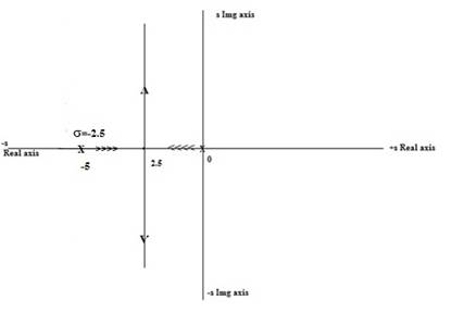
Fig.1
Conclusion:
Root has been plotted for the given characteristic equation is shown in Fig.1.
(b)
The root locus of the given characteristic equation
Explanation of Solution
Given:
Concept Used:
Root Locus technique.
Calculation:
The characteristic equation is defined as
Where,
Therefore, Poles are
And zero is
Total number of branches is
Centroid is calculated as:
Where poles are
Angle of asymptotes is calculated as:
Angle of asymptotes
Where P = no. of poles
Z = No. of zeros
On replacing the values
The
Breakaway point is calculated as:
To calculate breakaway point, replace
So,
Calculating the value of
For Stability
Auxiliary equation is defined as:
Replace the value of
For
For
This is the point on the imaginary axis
Angle of departure is calculated where there are either poles or zero is imaginary.
Root locus plot of the characteristic equation is
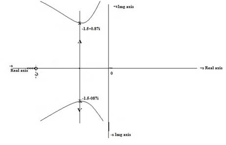
Fig.2
Conclusion:
Root has been plotted for the given characteristic equation is shown in Fig.2.
(c)
The root locus of the given characteristic equation
Explanation of Solution
Given:
Concept Used:
Root Locus technique.
Calculation:
The characteristic equation is defined as
Where,
Therefore, Poles are
And zero is
Total number of branches is
Centroid is calculated as:
Where poles are
Angle of asymptotes is calculated as:
Angle of asymptotes
Where P = no. of poles
Z = No. of zeros
On replacing the values
The
Breakaway point is calculated as:
To calculate breakaway point, replace
So,
Breakaway point is
Calculating the value of
For Stability
Auxiliary equation is defined as:
Replace the value of
This is the point on the imaginary axis
Root locus plot of the characteristic equation is
Fig.3
Conclusion:
Root has been plotted for the given characteristic equation is shown in Fig.3.
(d)
The root locus of the given characteristic equation
Explanation of Solution
Given:
Concept Used:
Root Locus technique.
Calculation:
The characteristic equation is defined as
On solving we get,
Therefore, Poles are
And zero is
Total number of branches is
Centroid is calculated as:
Where poles are
Angle of asymptotes is calculated as:
Angle of asymptotes
Where P = no. of poles
Z = No. of zeros
On replacing the values
The
Breakaway point is calculated as:
To calculate breakaway point, replace
So,
Breakaway point is
Calculating the value of
For Stability
Auxiliary equation is defined as:
Replace the value of
This is the point on the imaginary axis
Root locus plot of the characteristic equation is
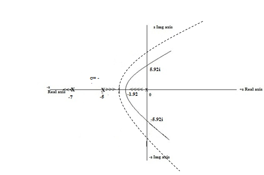
Fig.4
Conclusion:
Root has been plotted for the given characteristic equation is shown in Fig4.
(e)
The root locus of the given characteristic equation
Explanation of Solution
Given:
Concept Used:
Root Locus technique.
Calculation:
The characteristic equation is defined as
Where,
Therefore, Poles are
And zero is
Total number of branches is
Centroid is calculated as:
Where poles are
Angle of asymptotes is calculated as:
Angle of asymptotes
Where P = no. of poles
Z = No. of zeros
On replacing the values
The
Breakaway point is calculated as:
To calculate breakaway point, replace
So,
Breakaway point is
Calculating the value of
For Stability
Auxiliary equation is defined as:
Replace the value of
This is the point on the imaginary axis
Root locus plot of the characteristic equation is
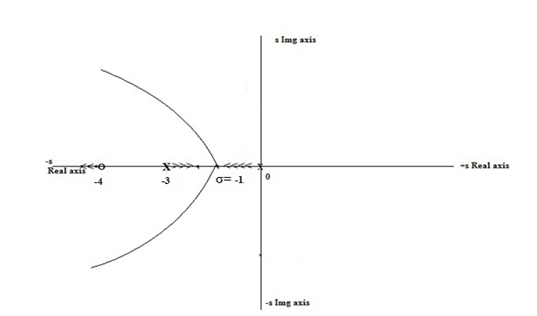
Fig.5
Conclusion:
Root has been plotted for the given characteristic equation is shown in Fig.5.
(f)
The root locus of the given characteristic equation
Explanation of Solution
Given:
Concept Used:
Root Locus technique.
Calculation:
The characteristic equation is defined as
Where,
Therefore, Poles are
And zero is
Total number of branches is
Centroid is calculated as:
Where poles are
Angle of asymptotes is calculated as:
Angle of asymptotes
Where P = no. of poles
Z = No. of zeros
On replacing the values
The
Breakaway point is calculated as:
To calculate breakaway point, replace
So,
Breakaway point is
Calculating the value of
For Stability
Auxiliary equation is defined as:
Replace the value of
For
For
Root locus plot of the characteristic equation is
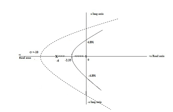
Fig.6
Conclusion:
Root has been plotted for the given characteristic equation is shown in Fig6.
Want to see more full solutions like this?
Chapter 11 Solutions
System Dynamics


- Consider radiation from a small surface at 100 oC which is enclosed by a much larger surface at24 o C. Determine the percent increase in the radiation heat transfer if the temperature of the smallsurface is doubled.arrow_forwardA small electronic package with a surface area of 820 cm2 is placed in a room where the airtemperature is 28 o C. The heat transfer coefficient is 7.3 W/m2 - o C. You are asked to determine if it isjustified to neglect heat loss from the package by radiation. Assume a uniform surface temperature of78 o C and surface emissivity of 0.65 Assume further that room’s walls and ceiling are at a uniformtemperature of 16 o C.arrow_forwardA hollow metal sphere of outer radius or = 2 cm is heated internally with a variable output electricheater. The sphere loses heat from its surface by convection and radiation. The heat transfercoefficient is 22 W/ m2 - o C and surface emissivity is 0.92. The ambient fluid temperature is 20 o C andthe surroundings temperature is 14 oC. Construct a graph of the surface temperature corresponding toheating rates ranging from zero to 100 watts. Assume steady state. Use a simplified model forradiation exchange based on a small gray surface enclosed by a much larger surface at 14 o C.arrow_forward
- 2. A program to make the part depicted in Figure 26.A has been created, presented in figure 26.B, but some information still needs to be filled in. Compute the tool locations, depths, and other missing information to present a completed program. (Hint: You may have to look up geometry for the center drill and standard 0.5000 in twist drill to know the required depth to drill). Dashed line indicates - corner of original stock Intended toolpath-tangent - arc entry and exit sized to programmer's judgment 026022 (Slot and Drill Part) (Setup Instructions. (UNITS: Inches (WORKPIECE MAT'L: SAE 1020 STEEL (Workpiece: 3.25 x 2.00 x0.75 in. Plate (PRZ Location G54: ( XY 0.0 Upper Left of Fixture ( TOP OF PART 2-0 (Tool List: ) ( T04 T02 0.500 IN 4 FLUTE FLAT END MILL) #4 CENTER DRILL ' T02 0.500 TWIST DRILL N010 GOO G90 G17 G20 G49 G40 G80 G54 N020 M06 T02 (0.5 IN 4-FLUTE END MILL) R0.750 N030 S760 M03 G00 x N040 043 H02 2 Y (P1) (RAPID DOWN -TLO) P4 NO50 MOB (COOLANT ON) N060 G01 X R1.000 N070…arrow_forward6–95. The reaction of the ballast on the railway tie can be assumed uniformly distributed over its length as shown. If the wood has an allowable bending stress of σallow=1.5 ksi, determine the required minimum thickness t of the rectangular cross section of the tie to the nearest 18 in. Please include all steps. Also if you can, please explain how you found Mmax using an equation rather than using just the moment diagram. Thank you!arrow_forward6–53. If the moment acting on the cross section is M=600 N⋅m, determine the resultant force the bending stress produces on the top board. Please explain each step. Please explain how you got the numbers and where you plugged them in to solve the problem. Thank you!arrow_forward
- Solving coplanar forcesarrow_forwardComplete the following problems. Show your work/calculations, save as.pdf and upload to the assignment in Blackboard. 1. What are the x and y dimensions for the center position of holes 1,2, and 3 in the part shown in Figure 26.2 (below)? 6.0000 7118 Zero reference point 1.0005 1.0000 1.252 Bore C' bore 1.250 6.0000 .7118 0.2180 deep (3 holes) 2.6563 1.9445 3.000 diam. slot 0.3000 deep. 0.3000 wide 2.6563 1.9445arrow_forwardComplete the following problems. Show your work/calculations, save as.pdf and upload to the assignment in Blackboard. missing information to present a completed program. (Hint: You may have to look up geometry for the center drill and standard 0.5000 in twist drill to know the required depth to drill). 1. What are the x and y dimensions for the center position of holes 1,2, and 3 in the part shown in Figure 26.2 (below)? 6.0000 Zero reference point 7118 1.0005 1.0000 1.252 Bore 6.0000 .7118 Cbore 0.2180 deep (3 holes) 2.6563 1.9445 Figure 26.2 026022 (8lot and Drill Part) (Setup Instructions--- (UNITS: Inches (WORKPIECE NAT'L SAE 1020 STEEL (Workpiece: 3.25 x 2.00 x0.75 in. Plate (PRZ Location 054: ' XY 0.0 - Upper Left of Fixture TOP OF PART 2-0 (Tool List ( T02 0.500 IN 4 FLUTE FLAT END MILL #4 CENTER DRILL Dashed line indicates- corner of original stock ( T04 T02 3.000 diam. slot 0.3000 deep. 0.3000 wide Intended toolpath-tangent- arc entry and exit sized to programmer's judgment…arrow_forward
- A program to make the part depicted in Figure 26.A has been created, presented in figure 26.B, but some information still needs to be filled in. Compute the tool locations, depths, and other missing information to present a completed program. (Hint: You may have to look up geometry for the center drill and standard 0.5000 in twist drill to know the required depth to drill).arrow_forwardWe consider a laminar flow induced by an impulsively started infinite flat plate. The y-axis is normal to the plate. The x- and z-axes form a plane parallel to the plate. The plate is defined by y = 0. For time t <0, the plate and the flow are at rest. For t≥0, the velocity of the plate is parallel to the 2-coordinate; its value is constant and equal to uw. At infinity, the flow is at rest. The flow induced by the motion of the plate is independent of z. (a) From the continuity equation, show that v=0 everywhere in the flow and the resulting momentum equation is მu Ət Note that this equation has the form of a diffusion equation (the same form as the heat equation). (b) We introduce the new variables T, Y and U such that T=kt, Y=k/2y, U = u where k is an arbitrary constant. In the new system of variables, the solution is U(Y,T). The solution U(Y,T) is expressed by a function of Y and T and the solution u(y, t) is expressed by a function of y and t. Show that the functions are identical.…arrow_forwardPart A: Suppose you wanted to drill a 1.5 in diameter hole through a piece of 1020 cold-rolled steel that is 2 in thick, using an HSS twist drill. What values if feed and cutting speed will you specify, along with an appropriate allowance? Part B: How much time will be required to drill the hole in the previous problem using the HSS drill?arrow_forward
 Elements Of ElectromagneticsMechanical EngineeringISBN:9780190698614Author:Sadiku, Matthew N. O.Publisher:Oxford University Press
 Mechanics of Materials (10th Edition)Mechanical EngineeringISBN:9780134319650Author:Russell C. HibbelerPublisher:PEARSON
 Thermodynamics: An Engineering ApproachMechanical EngineeringISBN:9781259822674Author:Yunus A. Cengel Dr., Michael A. BolesPublisher:McGraw-Hill Education
 Control Systems EngineeringMechanical EngineeringISBN:9781118170519Author:Norman S. NisePublisher:WILEY
 Mechanics of Materials (MindTap Course List)Mechanical EngineeringISBN:9781337093347Author:Barry J. Goodno, James M. GerePublisher:Cengage Learning
 Engineering Mechanics: StaticsMechanical EngineeringISBN:9781118807330Author:James L. Meriam, L. G. Kraige, J. N. BoltonPublisher:WILEY