Concept explainers
Videos
(a)
Section 1:
To graph: A
(a)
Section 1:
Explanation of Solution
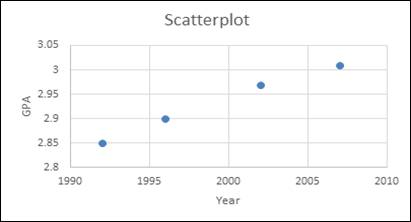
Graph: Plot the data from the provided table with GPA on y-axis and Year on x-axis.
Hence, the obtained graph is shown below:
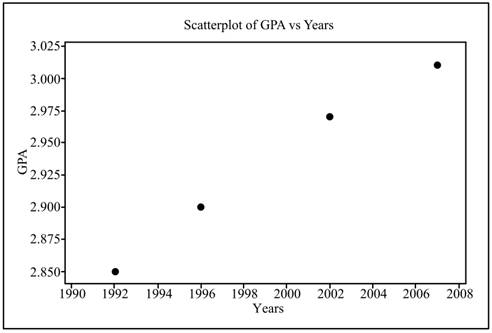
Interpretation: From the scatterplot, it can be seen that there is a linear dependency between GPA and year, which infers that the linear increase appears reasonable.
Section 2:
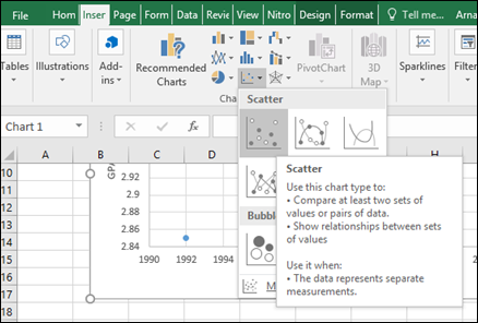
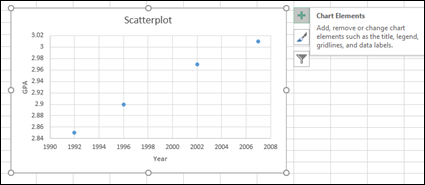
To graph: A scatterplot that shows the increase in GPA over time by using software and check whether the linear increase seems reasonable.
Section 2:
Explanation of Solution
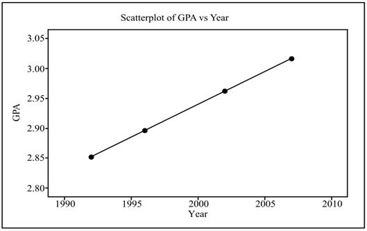
Graph: Construct a scatterplot using excel as follows:
Step 1: Enter the data in Excel.
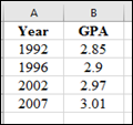
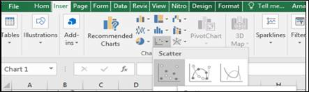
Step 2: Select the data. Click on Insert
Hence, the obtained graph is shown below:
Interpretation: From the scatterplot, it can be seen that there is a linear dependency between GPA and year, so it can be said that by using software the results are same.
(b)
Section 1:
To find: The least square regression line for predicting GPA from year by hand.
(b)
Section 1:
Answer to Problem 30E
Solution: The regression line is
Explanation of Solution
Calculation: Compute the value of
Now, compute
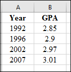
Year (x) |
GPA (y) |
xy |
x2 |
1992 |
2.85 |
5677.2 |
3968064 |
1996 |
2.90 |
5788.4 |
3984016 |
2002 |
2.97 |
5945.9 |
4008004 |
2007 |
3.01 |
6041.1 |
4028049 |
Now, compute the value of
Compute the value of
Now, compute the value of
Hence, the obtained regression equation is
Interpretation: Therefore, it can be concluded from the obtained regression equation that the GPA increases by 0.011 times with the increase in year.
Section 2:
To graph: A scatterplot that shows the fitting of least-squares regression line by hand.
Section 2:
Explanation of Solution
Calculation: Obtain points for plotting on the graph using the regression equation as follows:
Let
Let
Let
Let
Now, plot these points of GPA on
Graph:
Interpretation: Therefore, it can be said that all the points lie on the regression line, so it can be concluded that the line is a good fit.
Section 3:
To find: The least square regression line for predicting GPA from year by software.
Section 3:
Answer to Problem 30E
Solution: The regression line is:
Explanation of Solution
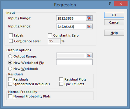
Calculation: Obtain the regression line using Excel as follows:
Step 1: Click on Data
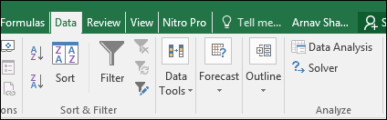
Step 3: Enter Y variable and X variable input
Step 4: Click ‘Ok’ to obtain the result.
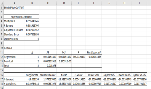
Hence, the obtained regression line is shown below:
Interpretation: Therefore, it can be concluded that the regression equation obtained by hand and software are approximately same.
Section 4:
To graph: A scatterplot which shows the fitting of least-squares regression line by software.
Section 4:
Explanation of Solution
Graph: Construct a scatterplot using excel as follows:
Step 1: Enter the data in Excel.
Step 2: Select the data. Click on Insert
Step 3: Now, put the cursor on the graph and a plus sign appears on the right hand side.
Step 4: Click on the plus sign and check the box for trend line.
Hence, the obtained graph is shown below:
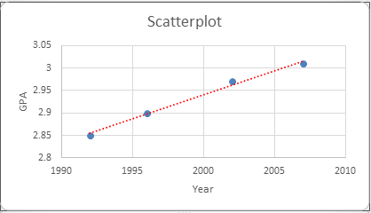
Interpretation: From the scatterplot, it can be seen that there is a linear dependency between GPA and year.
(c)
Section 1:
To find: The 95% confidence interval for the slope by hand.
(c)
Section 1:
Answer to Problem 30E
Solution: The confidence interval is
Explanation of Solution
Calculation: Now, compute
Year (x) |
GPA (y) |
|||
1992 |
2.85 |
2.852 |
0.000004 |
52.5625 |
1996 |
2.90 |
2.896 |
0.000016 |
10.5625 |
2002 |
2.97 |
2.962 |
0.000064 |
7.5625 |
2007 |
3.01 |
3.017 |
0.000049 |
60.0625 |
Now, compute the standard error of slope of regression
For 5% level of significance and
Compute the confidence interval as follows:
Interpretation: It can be said with 95% confidence that the GPA will increase between 0.008 and 0.014 over the time.
Section 2:
To find: The 95% confidence interval for the slope by software.
Section 2:
Answer to Problem 30E
Solution: The confidence interval is
Explanation of Solution
Calculation: Obtain the regression line using Excel as follows:
Step 1: Click on Data
Step 3: Enter Y variable and X variable input range.
Step 4: Click ‘Ok’ to obtain the result.
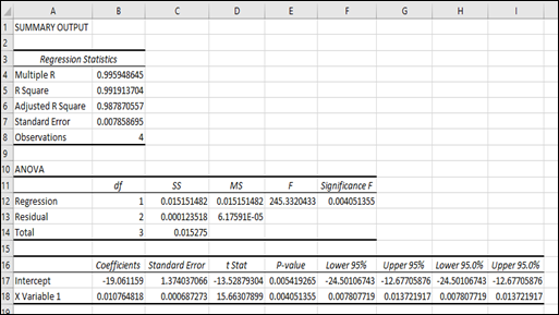
Hence, the obtained confidence interval for
Interpretation: Therefore, it can be concluded that the 95% confidence interval obtained by hand matched with the 95% confidence interval obtained by software.
Want to see more full solutions like this?
Chapter 10 Solutions
Introduction to the Practice of Statistics


- Question: A company launches two different marketing campaigns to promote the same product in two different regions. After one month, the company collects the sales data (in units sold) from both regions to compare the effectiveness of the campaigns. The company wants to determine whether there is a significant difference in the mean sales between the two regions. Perform a two sample T-test You can provide your answer by inserting a text box and the answer must include: Null hypothesis, Alternative hypothesis, Show answer (output table/summary table), and Conclusion based on the P value. (2 points = 0.5 x 4 Answers) Each of these is worth 0.5 points. However, showing the calculation is must. If calculation is missing, the whole answer won't get any credit.arrow_forwardBinomial Prob. Question: A new teaching method claims to improve student engagement. A survey reveals that 60% of students find this method engaging. If 15 students are randomly selected, what is the probability that: a) Exactly 9 students find the method engaging?b) At least 7 students find the method engaging? (2 points = 1 x 2 answers) Provide answers in the yellow cellsarrow_forwardIn a survey of 2273 adults, 739 say they believe in UFOS. Construct a 95% confidence interval for the population proportion of adults who believe in UFOs. A 95% confidence interval for the population proportion is ( ☐, ☐ ). (Round to three decimal places as needed.)arrow_forward
- Find the minimum sample size n needed to estimate μ for the given values of c, σ, and E. C=0.98, σ 6.7, and E = 2 Assume that a preliminary sample has at least 30 members. n = (Round up to the nearest whole number.)arrow_forwardIn a survey of 2193 adults in a recent year, 1233 say they have made a New Year's resolution. Construct 90% and 95% confidence intervals for the population proportion. Interpret the results and compare the widths of the confidence intervals. The 90% confidence interval for the population proportion p is (Round to three decimal places as needed.) J.D) .arrow_forwardLet p be the population proportion for the following condition. Find the point estimates for p and q. In a survey of 1143 adults from country A, 317 said that they were not confident that the food they eat in country A is safe. The point estimate for p, p, is (Round to three decimal places as needed.) ...arrow_forward
- (c) Because logistic regression predicts probabilities of outcomes, observations used to build a logistic regression model need not be independent. A. false: all observations must be independent B. true C. false: only observations with the same outcome need to be independent I ANSWERED: A. false: all observations must be independent. (This was marked wrong but I have no idea why. Isn't this a basic assumption of logistic regression)arrow_forwardBusiness discussarrow_forwardSpam filters are built on principles similar to those used in logistic regression. We fit a probability that each message is spam or not spam. We have several variables for each email. Here are a few: to_multiple=1 if there are multiple recipients, winner=1 if the word 'winner' appears in the subject line, format=1 if the email is poorly formatted, re_subj=1 if "re" appears in the subject line. A logistic model was fit to a dataset with the following output: Estimate SE Z Pr(>|Z|) (Intercept) -0.8161 0.086 -9.4895 0 to_multiple -2.5651 0.3052 -8.4047 0 winner 1.5801 0.3156 5.0067 0 format -0.1528 0.1136 -1.3451 0.1786 re_subj -2.8401 0.363 -7.824 0 (a) Write down the model using the coefficients from the model fit.log_odds(spam) = -0.8161 + -2.5651 + to_multiple + 1.5801 winner + -0.1528 format + -2.8401 re_subj(b) Suppose we have an observation where to_multiple=0, winner=1, format=0, and re_subj=0. What is the predicted probability that this message is spam?…arrow_forward
- Consider an event X comprised of three outcomes whose probabilities are 9/18, 1/18,and 6/18. Compute the probability of the complement of the event. Question content area bottom Part 1 A.1/2 B.2/18 C.16/18 D.16/3arrow_forwardJohn and Mike were offered mints. What is the probability that at least John or Mike would respond favorably? (Hint: Use the classical definition.) Question content area bottom Part 1 A.1/2 B.3/4 C.1/8 D.3/8arrow_forwardThe details of the clock sales at a supermarket for the past 6 weeks are shown in the table below. The time series appears to be relatively stable, without trend, seasonal, or cyclical effects. The simple moving average value of k is set at 2. What is the simple moving average root mean square error? Round to two decimal places. Week Units sold 1 88 2 44 3 54 4 65 5 72 6 85 Question content area bottom Part 1 A. 207.13 B. 20.12 C. 14.39 D. 0.21arrow_forward
 MATLAB: An Introduction with ApplicationsStatisticsISBN:9781119256830Author:Amos GilatPublisher:John Wiley & Sons Inc
 Probability and Statistics for Engineering and th...StatisticsISBN:9781305251809Author:Jay L. DevorePublisher:Cengage Learning
 Statistics for The Behavioral Sciences (MindTap C...StatisticsISBN:9781305504912Author:Frederick J Gravetter, Larry B. WallnauPublisher:Cengage Learning
 Elementary Statistics: Picturing the World (7th E...StatisticsISBN:9780134683416Author:Ron Larson, Betsy FarberPublisher:PEARSON
 The Basic Practice of StatisticsStatisticsISBN:9781319042578Author:David S. Moore, William I. Notz, Michael A. FlignerPublisher:W. H. Freeman
 Introduction to the Practice of StatisticsStatisticsISBN:9781319013387Author:David S. Moore, George P. McCabe, Bruce A. CraigPublisher:W. H. Freeman