
Concept explainers
Videos
(a)
Section 1:
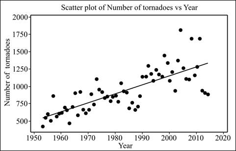
To graph: A
(a)
Section 1:
Explanation of Solution
Graph: Construct a scatterplot using Minitab as follows:
Step 1: Enter the data in Minitab.
Step 2: Click on Graph --> Scatterplot. Select scatterplot with regression.
Step 3: Double click on ‘Number of tornadoes’ to move it to Y variable and ‘Year’ to move it to X variable column.
Step 4: Click ‘Ok’ twice to obtain the graph.
Section 2:
To explain: The relationship between two variables seems linear.
Section 2:
Answer to Problem 19E
Solution: The variables are in linear relationship.
Explanation of Solution
Section 3:
To explain: Whether there are any outliers or unusual pattern.
Section 3:
Answer to Problem 19E
Solution: There are no outliers.
Explanation of Solution
(b)
To find: The least square regression line.
(b)
Answer to Problem 19E
Solution: The regression line is:
Explanation of Solution
Calculation: Obtain the regression line using Minitab as follows:
Step 1: Enter the data in Minitab.
Step 2: Click on Stat --> Regression --> Regression.
Step 3: Double click on ‘Number of tornadoes’ to move it to Y variable and ‘Year’ to move it to X variable column.
Step 4: Click on ‘Storage’ and check the box for residuals.
Step 5: Click ‘Ok’ twice to obtain the result.
Hence, the obtained regression line is
(c)
To explain: The intercept of regression equation.
(c)
Answer to Problem 19E
Solution: The fit is correct because intercept is only used when
Explanation of Solution
(d)
Section 1:
To find: The residuals.
(d)
Section 1:
Answer to Problem 19E
Solution: The residuals are as follows:
Years |
Number of tornadoes |
Residuals |
1953 |
421 |
-127.661 |
1954 |
550 |
-11.495 |
1955 |
593 |
18.670 |
1956 |
504 |
-83.164 |
1957 |
856 |
256.001 |
1958 |
564 |
-48.833 |
1959 |
604 |
-21.668 |
1960 |
616 |
-22.502 |
1961 |
697 |
45.663 |
1962 |
657 |
-7.171 |
1963 |
464 |
-213.006 |
1964 |
704 |
14.160 |
1965 |
906 |
203.325 |
1966 |
585 |
-130.509 |
1967 |
926 |
197.656 |
1968 |
660 |
-81.178 |
1969 |
608 |
-146.013 |
1970 |
653 |
-113.847 |
1971 |
888 |
108.318 |
1972 |
741 |
-51.516 |
1973 |
1102 |
296.649 |
1974 |
947 |
128.815 |
1975 |
920 |
88.980 |
1976 |
835 |
-8.854 |
1977 |
852 |
-4.689 |
1978 |
788 |
-81.523 |
1979 |
852 |
-30.358 |
1980 |
866 |
-29.192 |
1981 |
783 |
-125.027 |
1982 |
1046 |
125.139 |
1983 |
931 |
-2.696 |
1984 |
907 |
-39.530 |
1985 |
684 |
-275.365 |
1986 |
764 |
-208.199 |
1987 |
656 |
-329.034 |
1988 |
702 |
-295.868 |
1989 |
856 |
-154.703 |
1990 |
1133 |
109.463 |
1991 |
1132 |
95.628 |
1992 |
1298 |
248.794 |
1993 |
1176 |
113.959 |
1994 |
1082 |
7.125 |
1995 |
1235 |
147.290 |
1996 |
1173 |
72.456 |
1997 |
1148 |
34.621 |
1998 |
1449 |
322.787 |
1999 |
1340 |
200.952 |
2000 |
1075 |
-76.882 |
2001 |
1215 |
50.283 |
2002 |
934 |
-243.551 |
2003 |
1374 |
183.614 |
2004 |
1817 |
613.780 |
2005 |
1265 |
48.945 |
2006 |
1103 |
-125.889 |
2007 |
1096 |
-145.724 |
2008 |
1692 |
437.442 |
2009 |
1156 |
-111.393 |
2010 |
1282 |
1.773 |
2011 |
1691 |
397.938 |
2012 |
938 |
-367.896 |
2013 |
907 |
-411.731 |
2014 |
888 |
-443.565 |
Explanation of Solution
Calculation: Obtain the residuals using Minitab as follows:
Step 1: Enter the data in Minitab.
Step 2: Click on Stat --> Regression --> Regression.
Step 3: Double click on ‘Number of tornadoes’ to move it response column and ‘Year’ to move it to predictor column.
Step 4: Click on ‘Storage’ and check the box for residuals.
Step 5: Click ‘Ok’ to obtain the result.
Hence, the obtained residuals are shown below:
Years |
Number of tornadoes |
Residuals |
1953 |
421 |
-127.661 |
1954 |
550 |
-11.495 |
1955 |
593 |
18.670 |
1956 |
504 |
-83.164 |
1957 |
856 |
256.001 |
1958 |
564 |
-48.833 |
1959 |
604 |
-21.668 |
1960 |
616 |
-22.502 |
1961 |
697 |
45.663 |
1962 |
657 |
-7.171 |
1963 |
464 |
-213.006 |
1964 |
704 |
14.160 |
1965 |
906 |
203.325 |
1966 |
585 |
-130.509 |
1967 |
926 |
197.656 |
1968 |
660 |
-81.178 |
1969 |
608 |
-146.013 |
1970 |
653 |
-113.847 |
1971 |
888 |
108.318 |
1972 |
741 |
-51.516 |
1973 |
1102 |
296.649 |
1974 |
947 |
128.815 |
1975 |
920 |
88.980 |
1976 |
835 |
-8.854 |
1977 |
852 |
-4.689 |
1978 |
788 |
-81.523 |
1979 |
852 |
-30.358 |
1980 |
866 |
-29.192 |
1981 |
783 |
-125.027 |
1982 |
1046 |
125.139 |
1983 |
931 |
-2.696 |
1984 |
907 |
-39.530 |
1985 |
684 |
-275.365 |
1986 |
764 |
-208.199 |
1987 |
656 |
-329.034 |
1988 |
702 |
-295.868 |
1989 |
856 |
-154.703 |
1990 |
1133 |
109.463 |
1991 |
1132 |
95.628 |
1992 |
1298 |
248.794 |
1993 |
1176 |
113.959 |
1994 |
1082 |
7.125 |
1995 |
1235 |
147.290 |
1996 |
1173 |
72.456 |
1997 |
1148 |
34.621 |
1998 |
1449 |
322.787 |
1999 |
1340 |
200.952 |
2000 |
1075 |
-76.882 |
2001 |
1215 |
50.283 |
2002 |
934 |
-243.551 |
2003 |
1374 |
183.614 |
2004 |
1817 |
613.780 |
2005 |
1265 |
48.945 |
2006 |
1103 |
-125.889 |
2007 |
1096 |
-145.724 |
2008 |
1692 |
437.442 |
2009 |
1156 |
-111.393 |
2010 |
1282 |
1.773 |
2011 |
1691 |
397.938 |
2012 |
938 |
-367.896 |
2013 |
907 |
-411.731 |
2014 |
888 |
-443.565 |
Section 2:
To graph: The scatterplot of residual versus year.
Section 2:
Explanation of Solution
Graph: Construct a scatterplot using Minitab as follows:
Step 1: Enter the data in Minitab.
Step 2: Click on Graph --> Scatterplot. Select scatterplot with regression.
Step 3: Double click on ‘Residuals’ to move it to Y variable and ‘Year’ to move it to X variable column.
Step 4: Click ‘Ok’ to obtain the graph.
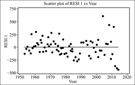
From the scatter plot, it is clear that the residual plot looks mostly random
(e)
To explain: That residuals are normal or not.
(e)
Answer to Problem 19E
Solution: The residuals are
Explanation of Solution
Graph: Construct the probability plot for residuals to test for the normality using Minitab as follows:
Step 1: Click on Stat -->
Step 2: Double click on ‘Residuals’ to move it to the variable column.
Step 3: Click ‘OK’ to obtain the graph.
Hence, the obtained graph is shown below:
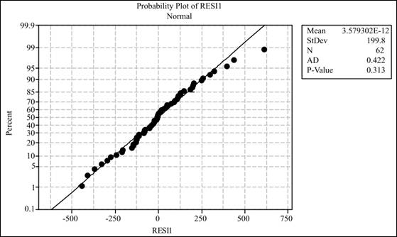
Interpretation: All the points lie near the trend line. Therefore, it can be concluded that residuals are normally distributed.
(f)
To explain: The accuracy of inference based on residual checks.
(f)
Answer to Problem 19E
Solution: The inference can be made based on residuals.
Explanation of Solution
Want to see more full solutions like this?
Chapter 10 Solutions
Introduction to the Practice of Statistics


- A marketing agency wants to determine whether different advertising platforms generate significantly different levels of customer engagement. The agency measures the average number of daily clicks on ads for three platforms: Social Media, Search Engines, and Email Campaigns. The agency collects data on daily clicks for each platform over a 10-day period and wants to test whether there is a statistically significant difference in the mean number of daily clicks among these platforms. Conduct ANOVA test. You can provide your answer by inserting a text box and the answer must include: also please provide a step by on getting the answers in excel Null hypothesis, Alternative hypothesis, Show answer (output table/summary table), and Conclusion based on the P value.arrow_forwardA company found that the daily sales revenue of its flagship product follows a normal distribution with a mean of $4500 and a standard deviation of $450. The company defines a "high-sales day" that is, any day with sales exceeding $4800. please provide a step by step on how to get the answers Q: What percentage of days can the company expect to have "high-sales days" or sales greater than $4800? Q: What is the sales revenue threshold for the bottom 10% of days? (please note that 10% refers to the probability/area under bell curve towards the lower tail of bell curve) Provide answers in the yellow cellsarrow_forwardBusiness Discussarrow_forward
- The following data represent total ventilation measured in liters of air per minute per square meter of body area for two independent (and randomly chosen) samples. Analyze these data using the appropriate non-parametric hypothesis testarrow_forwardeach column represents before & after measurements on the same individual. Analyze with the appropriate non-parametric hypothesis test for a paired design.arrow_forwardShould you be confident in applying your regression equation to estimate the heart rate of a python at 35°C? Why or why not?arrow_forward
 MATLAB: An Introduction with ApplicationsStatisticsISBN:9781119256830Author:Amos GilatPublisher:John Wiley & Sons Inc
 Probability and Statistics for Engineering and th...StatisticsISBN:9781305251809Author:Jay L. DevorePublisher:Cengage Learning
 Statistics for The Behavioral Sciences (MindTap C...StatisticsISBN:9781305504912Author:Frederick J Gravetter, Larry B. WallnauPublisher:Cengage Learning
 Elementary Statistics: Picturing the World (7th E...StatisticsISBN:9780134683416Author:Ron Larson, Betsy FarberPublisher:PEARSON
 The Basic Practice of StatisticsStatisticsISBN:9781319042578Author:David S. Moore, William I. Notz, Michael A. FlignerPublisher:W. H. Freeman
 Introduction to the Practice of StatisticsStatisticsISBN:9781319013387Author:David S. Moore, George P. McCabe, Bruce A. CraigPublisher:W. H. Freeman