
Concept explainers
Videos
(a)
To find: The fitted regression line by considering the log values of number of tornadoes.
(a)
Answer to Problem 22E
Solution: The fitted regression line where the Year is the predictor and log values of number of tornadoes is the response variable is provided below:
The variable
Explanation of Solution
Calculation: The log values of number of tornadoes can be calculated by using Microsoft excel by following the steps given below:
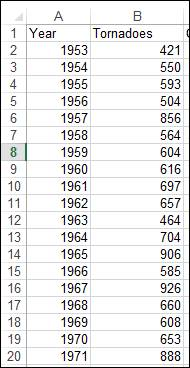
Step 1: Insert the data into the MS-Excel worksheet as shown in the screenshot below:
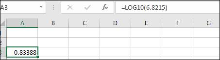
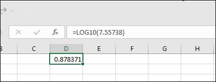
Step 2: Apply the formula to convert the number of tornadoes values to log values as displayed in the below screenshot:
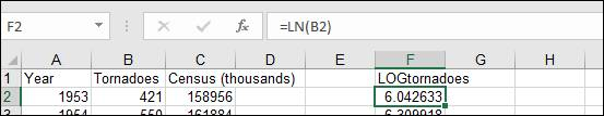
Step 3: Drag this output till the last cell of the total observation.
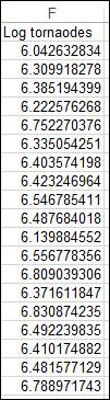
The log values are displayed in the screenshot below:
Further, the regression line can be fitted by using Minitab by following steps:
Step 1: Insert the data into the worksheet.
Step 2: Go to Stat
Step 3: Select LOGtornadoes in Response column and select Year in Predictors.
Step 4: Click “OK.”
After implementing these steps, the fitted regression line will appear in the output box, which is provided below:
Interpretation: The regression line concludes that as the year increases by a single quantity, it is expected that there will be an increase in the number of tornadoes by 1.41%.
(b)
To test: Whether the regression model fits the provided data.
(b)
Answer to Problem 22E
Solution: The residual plots for the Log tornadoes is provided below:

This plot represents that the assumptions for linear regression are valid.
Explanation of Solution
Calculation: The residuals along with the graph can be made by using the Minitab software by following the steps given below:
Step 1: Insert the data into the worksheet.
Step 2: Go to Stat
Step 3: Select LOGtornadoes in Response column and select Year in Predictors.
Step 4: Click on the button Storage and select Residuals.
Step 5: Click “OK.”
Step 6: Click on the button Graphs and select Four in one.
Step 7: Click “OK” twice.
After implementing these steps, a graph including four plots will appear in the output box and the column of residuals will add into the worksheet.
Some of the obtained residuals of the model are provided below:
Residuals |
0.331547 |
The plots are obtained as displayed below:
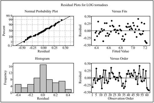
Conclusion: The normal probability plot shows that the residuals follows the normal distribution, residual versus fit plot shows that the residuals are randomly scattered, and the histogram shows that the residuals are symmetric. Hence the assumptions for linear regression analysis are reasonable.
(c)
To find: An approximate 95% confidence interval for percent change in the dependent variable.
(c)
Answer to Problem 22E
Solution: The 95% confidence interval for annual percent change in number of tornadoes is
Explanation of Solution
Given: The data for the annual number of Tornadoes in The United States from the year 1953 to 2014 are provided.
Calculation: The confidence interval can be calculated by using Minitab software by following the steps given below:
Step 1: Insert the data in the worksheet.
Step 2: Go to
Step 3: Click on the Results tab and select the Regression equation, Display confidence intervals and Prediction Tables options and click on “OK” twice to obtain the results.
The Minitab output displays the confidence interval as
(d)
To test: Whether this model supports the hypothesis of increment of tornadoes over the time.
(d)
Answer to Problem 22E
Solution: Yes, this model also supports the hypothesis that tornadoes have increased over the time.
Explanation of Solution
Given: The data for the annual number of Tornadoes in The United States from the year 1953 to 2014 are provided.
Calculation: To test the fact that whether tornadoes have increased over the time, the hypothesis are to be set as follows:
To test the above hypothesis, perform the following steps in Minitab:
Step 1: Insert the data in the Minitab worksheet.
Step 2: Go to Stat
Step 3: Click on the Results tab and select the Regression equation, Display confidence intervals and Prediction tables and click on “OK” twice to obtain the results.
After implementing these steps, P-value along with 95% confidence interval will appear in the output box for this model and the P-value obtained is 0.000, which is less than 0.05 and hence the null hypothesis is rejected at 5% level of significance.
Conclusion: Since the null hypothesis is rejected, it can be concluded that at 95% confidence level, the number of tornadoes have increased over the time.
(e)
To find: A prediction interval for number of tornadoes in the year 2015.
(e)
Answer to Problem 22E
Solution: The prediction interval for the number of tornadoes in the year 2015 is
Explanation of Solution
Calculation: The prediction interval for the number tornadoes in the year 2015 can be calculated by using the Minitab software by following the steps given below:
Step 1: Insert the data into the worksheet.
Step 2: Go to Stat
Step 3: Select logtornadoes in the Response column and Year in the Model column.
Step 4: Click on the button Prediction, write 2015 in the column of New observation for continuous prediction.
Step 5: In storage select Prediction limit and Confidence limit.
Step 6: Click “OK” twice to obtain the output.
After implementing these steps, the prediction interval will appear in the output box, which is
This model was fitted by taking the log values of the number of tornadoes, so the prediction interval has also been constructed for the log values. To get to know the actual prediction interval, antilog can be taken of the end points of this interval and anti-log can be calculated by using the software Microsoft excel as follows:
(f)
The model that is preferable, the one with the original number of tornadoes or the one with the log number of tornadoes.
(f)
Answer to Problem 22E
Solution: The model that was fitted by taking the natural logarithmic is preferable over the model, which was fitted by using the original values.
Explanation of Solution
Want to see more full solutions like this?
Chapter 10 Solutions
Introduction to the Practice of Statistics


- A marketing agency wants to determine whether different advertising platforms generate significantly different levels of customer engagement. The agency measures the average number of daily clicks on ads for three platforms: Social Media, Search Engines, and Email Campaigns. The agency collects data on daily clicks for each platform over a 10-day period and wants to test whether there is a statistically significant difference in the mean number of daily clicks among these platforms. Conduct ANOVA test. You can provide your answer by inserting a text box and the answer must include: also please provide a step by on getting the answers in excel Null hypothesis, Alternative hypothesis, Show answer (output table/summary table), and Conclusion based on the P value.arrow_forwardA company found that the daily sales revenue of its flagship product follows a normal distribution with a mean of $4500 and a standard deviation of $450. The company defines a "high-sales day" that is, any day with sales exceeding $4800. please provide a step by step on how to get the answers Q: What percentage of days can the company expect to have "high-sales days" or sales greater than $4800? Q: What is the sales revenue threshold for the bottom 10% of days? (please note that 10% refers to the probability/area under bell curve towards the lower tail of bell curve) Provide answers in the yellow cellsarrow_forwardBusiness Discussarrow_forward
- The following data represent total ventilation measured in liters of air per minute per square meter of body area for two independent (and randomly chosen) samples. Analyze these data using the appropriate non-parametric hypothesis testarrow_forwardeach column represents before & after measurements on the same individual. Analyze with the appropriate non-parametric hypothesis test for a paired design.arrow_forwardShould you be confident in applying your regression equation to estimate the heart rate of a python at 35°C? Why or why not?arrow_forward
 MATLAB: An Introduction with ApplicationsStatisticsISBN:9781119256830Author:Amos GilatPublisher:John Wiley & Sons Inc
 Probability and Statistics for Engineering and th...StatisticsISBN:9781305251809Author:Jay L. DevorePublisher:Cengage Learning
 Statistics for The Behavioral Sciences (MindTap C...StatisticsISBN:9781305504912Author:Frederick J Gravetter, Larry B. WallnauPublisher:Cengage Learning
 Elementary Statistics: Picturing the World (7th E...StatisticsISBN:9780134683416Author:Ron Larson, Betsy FarberPublisher:PEARSON
 The Basic Practice of StatisticsStatisticsISBN:9781319042578Author:David S. Moore, William I. Notz, Michael A. FlignerPublisher:W. H. Freeman
 Introduction to the Practice of StatisticsStatisticsISBN:9781319013387Author:David S. Moore, George P. McCabe, Bruce A. CraigPublisher:W. H. Freeman