Concept explainers
Videos
(a)
To find: The variables IBI and Forest using numerical method.
(a)
Answer to Problem 49E
Solution: The obtained result can be shown in tabular form as follows:
Variable |
Mean |
Standard deviation |
Forest |
39.39 |
32.20 |
IBI |
65.94 |
18.28 |
Explanation of Solution
Calculation: Calculate the average and standard deviation of IBI and Forest using Minitab as follows:
Step 1: Enter the data in Minitab.
Step 2: Go to Graphs > Histogram > Simple histogram.
Step 3: Double click on ‘Forest’ and ‘IBI’ to move it to variables column.
Step 4: Click on ‘Statistics’ and check the box for mean and standard deviation.
Step 5: Click ‘OK’ twice to obtain the result.
Results are obtained as:
Variable |
Mean |
Standard deviation |
Forest |
39.39 |
32.20 |
IBI |
65.94 |
18.28 |
To find: The variables IBI and Forest using graphical method.
Answer to Problem 49E
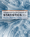
Solution: The graph of Forest is right skewed and the graph of IBI is left skewed.
Explanation of Solution
Graph: Construct the histograms to check the skewness using Minitab as follows:
Step 1: Click on Graphs --> Histogram. Select simple histogram.
Step 2: Double click on ‘Forest’ and ‘IBI’ to move it to variables column.
Step 3: Click ‘OK’ to obtain the result.
Interpretation: The graph of Forest is right skewed and the graph of IBI is left skewed.
(b)
To graph: A
(b)
Explanation of Solution
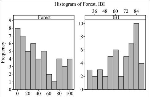
Graph: Construct a scatter plot as follows:
Step 1: Enter the data in Minitab.
Step 2: Click on Graph --> Scatterplot. Select scatterplot with regression.
Step 3: Double click on ‘BAC’ to move it Y variable and ‘Beer’ to move it to X variable column.
Step 4: Click ‘Ok’ twice to obtain the graph.
The scatter plot is obtained as:
Interpretation: The graph shows weak linear relationship between IBI and Forest with no unusual activity.
(c)
To explain: The statistical model for simple linear regression.
(c)
Answer to Problem 49E
Solution: The model is
Explanation of Solution
Where,
(d)
To explain: The null and alternate hypotheses.
(d)
Answer to Problem 49E
Solution: The null and alternative hypotheses are:
Explanation of Solution
So, the null and alternative hypothesis can be stated as:
(e)
To test: The least square
(e)
Answer to Problem 49E
Solution: The obtained output represents that the p-value is greater than 0.05. So there is no enough evidence for the linearity in the regression line.
Explanation of Solution
Calculation: Obtain the regression line using Minitab as follows:
Step 1: Enter the data in Minitab.
Step 2: Click on Stat --> Regression --> Regression.
Step 3: Double click on ‘IBI’ to move it response column and ‘Forest’ to move it to predictor column.
Step 4: Click ‘Ok’ to obtain the result.
Conclusion: From the obtained output the value of test statistic is 1.92 and the p-value is 0.061. Since the p-value is greater than 0.05, it can be concluded that there is no enough evidence for the linearity in the regression line
(f)
To find: The residuals.
(f)
Answer to Problem 49E
Solution: The residuals are as follows:
Forest |
IBI |
Residuals |
0 |
47 |
-12.9072 |
0 |
76 |
16.0928 |
9 |
33 |
-28.2854 |
17 |
78 |
15.4895 |
25 |
62 |
-1.7355 |
33 |
78 |
13.0394 |
47 |
33 |
-34.1045 |
59 |
64 |
-4.9420 |
79 |
83 |
10.9953 |
95 |
67 |
-7.4548 |
0 |
61 |
1.0928 |
3 |
85 |
24.6334 |
10 |
46 |
-15.4386 |
17 |
53 |
-9.5105 |
31 |
55 |
-9.6543 |
39 |
71 |
5.1206 |
49 |
59 |
-8.4107 |
63 |
41 |
-28.5546 |
80 |
82 |
9.8422 |
95 |
56 |
-18.4548 |
0 |
39 |
-20.9072 |
3 |
89 |
28.6334 |
10 |
32 |
-29.4386 |
18 |
43 |
-19.6636 |
32 |
29 |
-35.8075 |
41 |
55 |
-11.1857 |
49 |
81 |
13.5893 |
68 |
82 |
11.6798 |
86 |
82 |
8.9234 |
100 |
85 |
9.7795 |
0 |
59 |
-0.9072 |
7 |
74 |
13.0208 |
11 |
80 |
18.4083 |
21 |
88 |
24.8770 |
33 |
29 |
-35.9606 |
43 |
58 |
-8.4919 |
52 |
71 |
3.1299 |
75 |
60 |
-11.3922 |
89 |
86 |
12.4640 |
100 |
91 |
15.7795 |
0 |
72 |
12.0928 |
8 |
89 |
27.8677 |
14 |
80 |
17.9489 |
22 |
84 |
20.7238 |
33 |
54 |
-10.9606 |
43 |
71 |
4.5081 |
52 |
75 |
7.1299 |
79 |
84 |
11.9953 |
90 |
79 |
5.3109 |
Explanation of Solution
Calculation: Obtain the regression line using Minitab as follows:
Step 1: Enter the data in Minitab.
Step 2: Click on Stat --> Regression --> Regression.
Step 3: Double click on ‘IBI’ to move it response column and ‘Forest’ to move it to predictor column.
Step 4: Click on ‘Storage’ and check the box for residuals.
Step 5: Click ‘Ok’ twice to obtain the result.
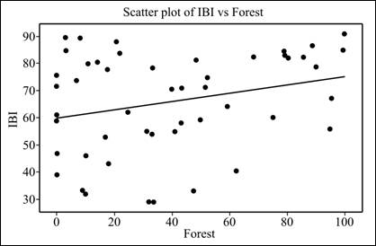
To graph: The scatterplot.
Explanation of Solution
Graph: Construct a scatterplot using Minitab as follows:
Step 1: Enter the data in Minitab.
Step 2: Click on Graph --> Scatterplot. Select scatterplot with regression.
Step 3: Double click on ‘Forest’ to move it X variable and ‘Residuals’ to move it to Y variable column.
Step 4: Click ‘Ok’ to obtain the graph.
The scatter plot is obtained as:
Interpretation: The graph shows that there is more variation for small
To explain: Whether there is something unusual.
Answer to Problem 49E
Solution: No, there is nothing unusual.
Explanation of Solution
(g)
To find: That residuals are normal or not.
(g)
Answer to Problem 49E
Solution: The residuals are approximately
Explanation of Solution
Step 1: Click on Stat -->
Step 2: Double click on ‘Residuals’ to move it to the variable column.
Step 3: Click ‘OK’ to obtain the graph.
The graph is obtained.
Interpretation: All the points lie near the trend line. Therefore, it can be concluded that residuals are approximately normally distributed.
(h)
To explain: If the assumptions of statistical inference in satisfied or not.
(h)
Answer to Problem 49E
Solution: The assumptions are not reasonable.
Explanation of Solution
Want to see more full solutions like this?
Chapter 10 Solutions
Introduction to the Practice of Statistics


- A smallish urn contains 25 small plastic bunnies – 7 of which are pink and 18 of which are white. 10 bunnies are drawn from the urn at random with replacement, and X is the number of pink bunnies that are drawn. (a) P(X = 5) ≈ (b) P(X<6) ≈ The Whoville small urn contains 100 marbles – 60 blue and 40 orange. The Grinch sneaks in one night and grabs a simple random sample (without replacement) of 15 marbles. (a) The probability that the Grinch gets exactly 6 blue marbles is [ Select ] ["≈ 0.054", "≈ 0.043", "≈ 0.061"] . (b) The probability that the Grinch gets at least 7 blue marbles is [ Select ] ["≈ 0.922", "≈ 0.905", "≈ 0.893"] . (c) The probability that the Grinch gets between 8 and 12 blue marbles (inclusive) is [ Select ] ["≈ 0.801", "≈ 0.760", "≈ 0.786"] . The Whoville small urn contains 100 marbles – 60 blue and 40 orange. The Grinch sneaks in one night and grabs a simple random sample (without replacement) of 15 marbles. (a)…arrow_forwardSuppose an experiment was conducted to compare the mileage(km) per litre obtained by competing brands of petrol I,II,III. Three new Mazda, three new Toyota and three new Nissan cars were available for experimentation. During the experiment the cars would operate under same conditions in order to eliminate the effect of external variables on the distance travelled per litre on the assigned brand of petrol. The data is given as below: Brands of Petrol Mazda Toyota Nissan I 10.6 12.0 11.0 II 9.0 15.0 12.0 III 12.0 17.4 13.0 (a) Test at the 5% level of significance whether there are signi cant differences among the brands of fuels and also among the cars. [10] (b) Compute the standard error for comparing any two fuel brands means. Hence compare, at the 5% level of significance, each of fuel brands II, and III with the standard fuel brand I. [10] �arrow_forwardBusiness discussarrow_forward
- What would you say about a set of quantitative bivariate data whose linear correlation is -1? What would a scatter diagram of the data look like? (5 points)arrow_forwardBusiness discussarrow_forwardAnalyze the residuals of a linear regression model and select the best response. yes, the residual plot does not show a curve no, the residual plot shows a curve yes, the residual plot shows a curve no, the residual plot does not show a curve I answered, "No, the residual plot shows a curve." (and this was incorrect). I am not sure why I keep getting these wrong when the answer seems obvious. Please help me understand what the yes and no references in the answer.arrow_forward
- a. Find the value of A.b. Find pX(x) and py(y).c. Find pX|y(x|y) and py|X(y|x)d. Are x and y independent? Why or why not?arrow_forwardAnalyze the residuals of a linear regression model and select the best response.Criteria is simple evaluation of possible indications of an exponential model vs. linear model) no, the residual plot does not show a curve yes, the residual plot does not show a curve yes, the residual plot shows a curve no, the residual plot shows a curve I selected: yes, the residual plot shows a curve and it is INCORRECT. Can u help me understand why?arrow_forwardYou have been hired as an intern to run analyses on the data and report the results back to Sarah; the five questions that Sarah needs you to address are given below. please do it step by step on excel Does there appear to be a positive or negative relationship between price and screen size? Use a scatter plot to examine the relationship. Determine and interpret the correlation coefficient between the two variables. In your interpretation, discuss the direction of the relationship (positive, negative, or zero relationship). Also discuss the strength of the relationship. Estimate the relationship between screen size and price using a simple linear regression model and interpret the estimated coefficients. (In your interpretation, tell the dollar amount by which price will change for each unit of increase in screen size). Include the manufacturer dummy variable (Samsung=1, 0 otherwise) and estimate the relationship between screen size, price and manufacturer dummy as a multiple…arrow_forward
- Here is data with as the response variable. x y54.4 19.124.9 99.334.5 9.476.6 0.359.4 4.554.4 0.139.2 56.354 15.773.8 9-156.1 319.2Make a scatter plot of this data. Which point is an outlier? Enter as an ordered pair, e.g., (x,y). (x,y)= Find the regression equation for the data set without the outlier. Enter the equation of the form mx+b rounded to three decimal places. y_wo= Find the regression equation for the data set with the outlier. Enter the equation of the form mx+b rounded to three decimal places. y_w=arrow_forwardYou have been hired as an intern to run analyses on the data and report the results back to Sarah; the five questions that Sarah needs you to address are given below. please do it step by step Does there appear to be a positive or negative relationship between price and screen size? Use a scatter plot to examine the relationship. Determine and interpret the correlation coefficient between the two variables. In your interpretation, discuss the direction of the relationship (positive, negative, or zero relationship). Also discuss the strength of the relationship. Estimate the relationship between screen size and price using a simple linear regression model and interpret the estimated coefficients. (In your interpretation, tell the dollar amount by which price will change for each unit of increase in screen size). Include the manufacturer dummy variable (Samsung=1, 0 otherwise) and estimate the relationship between screen size, price and manufacturer dummy as a multiple linear…arrow_forwardExercises: Find all the whole number solutions of the congruence equation. 1. 3x 8 mod 11 2. 2x+3= 8 mod 12 3. 3x+12= 7 mod 10 4. 4x+6= 5 mod 8 5. 5x+3= 8 mod 12arrow_forward
 MATLAB: An Introduction with ApplicationsStatisticsISBN:9781119256830Author:Amos GilatPublisher:John Wiley & Sons Inc
 Probability and Statistics for Engineering and th...StatisticsISBN:9781305251809Author:Jay L. DevorePublisher:Cengage Learning
 Statistics for The Behavioral Sciences (MindTap C...StatisticsISBN:9781305504912Author:Frederick J Gravetter, Larry B. WallnauPublisher:Cengage Learning
 Elementary Statistics: Picturing the World (7th E...StatisticsISBN:9780134683416Author:Ron Larson, Betsy FarberPublisher:PEARSON
 The Basic Practice of StatisticsStatisticsISBN:9781319042578Author:David S. Moore, William I. Notz, Michael A. FlignerPublisher:W. H. Freeman
 Introduction to the Practice of StatisticsStatisticsISBN:9781319013387Author:David S. Moore, George P. McCabe, Bruce A. CraigPublisher:W. H. Freeman