
Concept explainers
Videos
(a)
To find: The fitted regression line by considering the log values of number of tornadoes.
(a)
Answer to Problem 22E
Solution: The fitted regression line where the Year is the predictor and log values of number of tornadoes is the response variable is provided below:
The variable
Explanation of Solution
Calculation: The log values of number of tornadoes can be calculated by using Microsoft excel by following the steps given below:
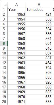
Step 1: Insert the data into the MS-Excel worksheet as shown in the screenshot below:
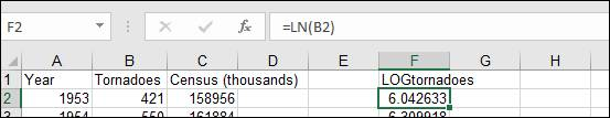
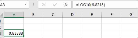
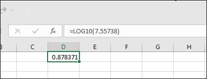
Step 2: Apply the formula to convert the number of tornadoes values to log values as displayed in the below screenshot:
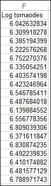
Step 3: Drag this output till the last cell of the total observation.
The log values are displayed in the screenshot below:
Further, the regression line can be fitted by using Minitab by following steps:
Step 1: Insert the data into the worksheet.
Step 2: Go to Stat
Step 3: Select LOGtornadoes in Response column and select Year in Predictors.
Step 4: Click “OK.”
After implementing these steps, the fitted regression line will appear in the output box, which is provided below:
Interpretation: The regression line concludes that as the year increases by a single quantity, it is expected that there will be an increase in the number of tornadoes by 1.41%.
(b)
To test: Whether the regression model fits the provided data.
(b)
Answer to Problem 22E
Solution: The residual plots for the Log tornadoes is provided below:

This plot represents that the assumptions for linear regression are valid.
Explanation of Solution
Calculation: The residuals along with the graph can be made by using the Minitab software by following the steps given below:
Step 1: Insert the data into the worksheet.
Step 2: Go to Stat
Step 3: Select LOGtornadoes in Response column and select Year in Predictors.
Step 4: Click on the button Storage and select Residuals.
Step 5: Click “OK.”
Step 6: Click on the button Graphs and select Four in one.
Step 7: Click “OK” twice.
After implementing these steps, a graph including four plots will appear in the output box and the column of residuals will add into the worksheet.
Some of the obtained residuals of the model are provided below:
Residuals |
0.331547 |
The plots are obtained as displayed below:
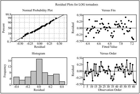
Conclusion: The normal probability plot shows that the residuals follows the normal distribution, residual versus fit plot shows that the residuals are randomly scattered, and the histogram shows that the residuals are symmetric. Hence the assumptions for linear regression analysis are reasonable.
(c)
To find: An approximate 95% confidence interval for percent change in the dependent variable.
(c)
Answer to Problem 22E
Solution: The 95% confidence interval for annual percent change in number of tornadoes is
Explanation of Solution
Given: The data for the annual number of Tornadoes in The United States from the year 1953 to 2014 are provided.
Calculation: The confidence interval can be calculated by using Minitab software by following the steps given below:
Step 1: Insert the data in the worksheet.
Step 2: Go to
Step 3: Click on the Results tab and select the Regression equation, Display confidence intervals and Prediction Tables options and click on “OK” twice to obtain the results.
The Minitab output displays the confidence interval as
(d)
To test: Whether this model supports the hypothesis of increment of tornadoes over the time.
(d)
Answer to Problem 22E
Solution: Yes, this model also supports the hypothesis that tornadoes have increased over the time.
Explanation of Solution
Given: The data for the annual number of Tornadoes in The United States from the year 1953 to 2014 are provided.
Calculation: To test the fact that whether tornadoes have increased over the time, the hypothesis are to be set as follows:
To test the above hypothesis, perform the following steps in Minitab:
Step 1: Insert the data in the Minitab worksheet.
Step 2: Go to Stat
Step 3: Click on the Results tab and select the Regression equation, Display confidence intervals and Prediction tables and click on “OK” twice to obtain the results.
After implementing these steps, P-value along with 95% confidence interval will appear in the output box for this model and the P-value obtained is 0.000, which is less than 0.05 and hence the null hypothesis is rejected at 5% level of significance.
Conclusion: Since the null hypothesis is rejected, it can be concluded that at 95% confidence level, the number of tornadoes have increased over the time.
(e)
To find: A prediction interval for number of tornadoes in the year 2015.
(e)
Answer to Problem 22E
Solution: The prediction interval for the number of tornadoes in the year 2015 is
Explanation of Solution
Calculation: The prediction interval for the number tornadoes in the year 2015 can be calculated by using the Minitab software by following the steps given below:
Step 1: Insert the data into the worksheet.
Step 2: Go to Stat
Step 3: Select logtornadoes in the Response column and Year in the Model column.
Step 4: Click on the button Prediction, write 2015 in the column of New observation for continuous prediction.
Step 5: In storage select Prediction limit and Confidence limit.
Step 6: Click “OK” twice to obtain the output.
After implementing these steps, the prediction interval will appear in the output box, which is
This model was fitted by taking the log values of the number of tornadoes, so the prediction interval has also been constructed for the log values. To get to know the actual prediction interval, antilog can be taken of the end points of this interval and anti-log can be calculated by using the software Microsoft excel as follows:
(f)
The model that is preferable, the one with the original number of tornadoes or the one with the log number of tornadoes.
(f)
Answer to Problem 22E
Solution: The model that was fitted by taking the natural logarithmic is preferable over the model, which was fitted by using the original values.
Explanation of Solution
Want to see more full solutions like this?
Chapter 10 Solutions
Introduction to the Practice of Statistics 9E & LaunchPad for Introduction to the Practice of Statistics 9E (Twelve-Month Access)


- The PDF of an amplitude X of a Gaussian signal x(t) is given by:arrow_forwardThe PDF of a random variable X is given by the equation in the picture.arrow_forwardFor a binary asymmetric channel with Py|X(0|1) = 0.1 and Py|X(1|0) = 0.2; PX(0) = 0.4 isthe probability of a bit of “0” being transmitted. X is the transmitted digit, and Y is the received digit.a. Find the values of Py(0) and Py(1).b. What is the probability that only 0s will be received for a sequence of 10 digits transmitted?c. What is the probability that 8 1s and 2 0s will be received for the same sequence of 10 digits?d. What is the probability that at least 5 0s will be received for the same sequence of 10 digits?arrow_forward
- V2 360 Step down + I₁ = I2 10KVA 120V 10KVA 1₂ = 360-120 or 2nd Ratio's V₂ m 120 Ratio= 360 √2 H I2 I, + I2 120arrow_forwardQ2. [20 points] An amplitude X of a Gaussian signal x(t) has a mean value of 2 and an RMS value of √(10), i.e. square root of 10. Determine the PDF of x(t).arrow_forwardIn a network with 12 links, one of the links has failed. The failed link is randomlylocated. An electrical engineer tests the links one by one until the failed link is found.a. What is the probability that the engineer will find the failed link in the first test?b. What is the probability that the engineer will find the failed link in five tests?Note: You should assume that for Part b, the five tests are done consecutively.arrow_forward
- Problem 3. Pricing a multi-stock option the Margrabe formula The purpose of this problem is to price a swap option in a 2-stock model, similarly as what we did in the example in the lectures. We consider a two-dimensional Brownian motion given by W₁ = (W(¹), W(2)) on a probability space (Q, F,P). Two stock prices are modeled by the following equations: dX = dY₁ = X₁ (rdt+ rdt+0₁dW!) (²)), Y₁ (rdt+dW+0zdW!"), with Xo xo and Yo =yo. This corresponds to the multi-stock model studied in class, but with notation (X+, Y₁) instead of (S(1), S(2)). Given the model above, the measure P is already the risk-neutral measure (Both stocks have rate of return r). We write σ = 0₁+0%. We consider a swap option, which gives you the right, at time T, to exchange one share of X for one share of Y. That is, the option has payoff F=(Yr-XT). (a) We first assume that r = 0 (for questions (a)-(f)). Write an explicit expression for the process Xt. Reminder before proceeding to question (b): Girsanov's theorem…arrow_forwardProblem 1. Multi-stock model We consider a 2-stock model similar to the one studied in class. Namely, we consider = S(1) S(2) = S(¹) exp (σ1B(1) + (M1 - 0/1 ) S(²) exp (02B(2) + (H₂- M2 where (B(¹) ) +20 and (B(2) ) +≥o are two Brownian motions, with t≥0 Cov (B(¹), B(2)) = p min{t, s}. " The purpose of this problem is to prove that there indeed exists a 2-dimensional Brownian motion (W+)+20 (W(1), W(2))+20 such that = S(1) S(2) = = S(¹) exp (011W(¹) + (μ₁ - 01/1) t) 롱) S(²) exp (021W (1) + 022W(2) + (112 - 03/01/12) t). where σ11, 21, 22 are constants to be determined (as functions of σ1, σ2, p). Hint: The constants will follow the formulas developed in the lectures. (a) To show existence of (Ŵ+), first write the expression for both W. (¹) and W (2) functions of (B(1), B(²)). as (b) Using the formulas obtained in (a), show that the process (WA) is actually a 2- dimensional standard Brownian motion (i.e. show that each component is normal, with mean 0, variance t, and that their…arrow_forwardThe scores of 8 students on the midterm exam and final exam were as follows. Student Midterm Final Anderson 98 89 Bailey 88 74 Cruz 87 97 DeSana 85 79 Erickson 85 94 Francis 83 71 Gray 74 98 Harris 70 91 Find the value of the (Spearman's) rank correlation coefficient test statistic that would be used to test the claim of no correlation between midterm score and final exam score. Round your answer to 3 places after the decimal point, if necessary. Test statistic: rs =arrow_forward
- Business discussarrow_forwardBusiness discussarrow_forwardI just need to know why this is wrong below: What is the test statistic W? W=5 (incorrect) and What is the p-value of this test? (p-value < 0.001-- incorrect) Use the Wilcoxon signed rank test to test the hypothesis that the median number of pages in the statistics books in the library from which the sample was taken is 400. A sample of 12 statistics books have the following numbers of pages pages 127 217 486 132 397 297 396 327 292 256 358 272 What is the sum of the negative ranks (W-)? 75 What is the sum of the positive ranks (W+)? 5What type of test is this? two tailedWhat is the test statistic W? 5 These are the critical values for a 1-tailed Wilcoxon Signed Rank test for n=12 Alpha Level 0.001 0.005 0.01 0.025 0.05 0.1 0.2 Critical Value 75 70 68 64 60 56 50 What is the p-value for this test? p-value < 0.001arrow_forward
 MATLAB: An Introduction with ApplicationsStatisticsISBN:9781119256830Author:Amos GilatPublisher:John Wiley & Sons Inc
 Probability and Statistics for Engineering and th...StatisticsISBN:9781305251809Author:Jay L. DevorePublisher:Cengage Learning
 Statistics for The Behavioral Sciences (MindTap C...StatisticsISBN:9781305504912Author:Frederick J Gravetter, Larry B. WallnauPublisher:Cengage Learning
 Elementary Statistics: Picturing the World (7th E...StatisticsISBN:9780134683416Author:Ron Larson, Betsy FarberPublisher:PEARSON
 The Basic Practice of StatisticsStatisticsISBN:9781319042578Author:David S. Moore, William I. Notz, Michael A. FlignerPublisher:W. H. Freeman
 Introduction to the Practice of StatisticsStatisticsISBN:9781319013387Author:David S. Moore, George P. McCabe, Bruce A. CraigPublisher:W. H. Freeman