
Concept explainers
Videos
(a)
Section 1:
To graph: A
(a)
Section 1:
Explanation of Solution
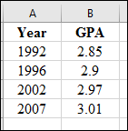
Graph: Plot the data from the provided table with GPA on y-axis and Year on x-axis.
Hence, the obtained graph is shown below:
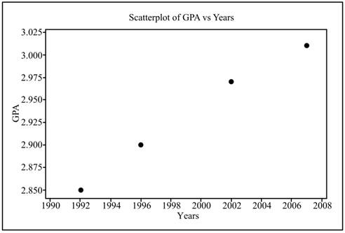
Interpretation: From the scatterplot, it can be seen that there is a linear dependency between GPA and year, which infers that the linear increase appears reasonable.
Section 2:
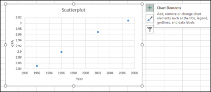
To graph: A scatterplot that shows the increase in GPA over time by using software and check whether the linear increase seems reasonable.
Section 2:
Explanation of Solution
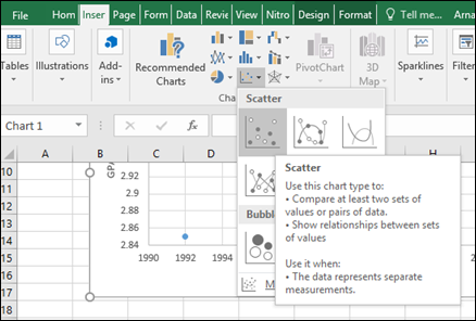
Graph: Construct a scatterplot using excel as follows:
Step 1: Enter the data in Excel.
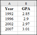
Step 2: Select the data. Click on Insert

Hence, the obtained graph is shown below:
Interpretation: From the scatterplot, it can be seen that there is a linear dependency between GPA and year, so it can be said that by using software the results are same.
(b)
Section 1:
To find: The least square regression line for predicting GPA from year by hand.
(b)
Section 1:
Answer to Problem 30E
Solution: The regression line is
Explanation of Solution
Calculation: Compute the value of
Now, compute
Year (x) |
GPA (y) |
xy |
x2 |
1992 |
2.85 |
5677.2 |
3968064 |
1996 |
2.90 |
5788.4 |
3984016 |
2002 |
2.97 |
5945.9 |
4008004 |
2007 |
3.01 |
6041.1 |
4028049 |
Now, compute the value of
Compute the value of
Now, compute the value of
Hence, the obtained regression equation is
Interpretation: Therefore, it can be concluded from the obtained regression equation that the GPA increases by 0.011 times with the increase in year.
Section 2:
To graph: A scatterplot that shows the fitting of least-squares regression line by hand.
Section 2:
Explanation of Solution
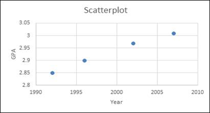
Calculation: Obtain points for plotting on the graph using the regression equation as follows:
Let
Let
Let
Let
Now, plot these points of GPA on
Graph:
Interpretation: Therefore, it can be said that all the points lie on the regression line, so it can be concluded that the line is a good fit.
Section 3:
To find: The least square regression line for predicting GPA from year by software.
Section 3:
Answer to Problem 30E
Solution: The regression line is:
Explanation of Solution
Calculation: Obtain the regression line using Excel as follows:
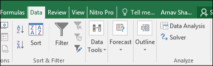
Step 1: Click on Data
Step 3: Enter Y variable and X variable input
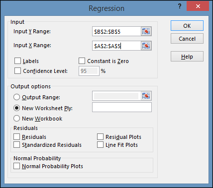
Step 4: Click ‘Ok’ to obtain the result.
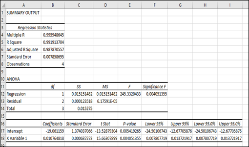
Hence, the obtained regression line is shown below:
Interpretation: Therefore, it can be concluded that the regression equation obtained by hand and software are approximately same.
Section 4:
To graph: A scatterplot which shows the fitting of least-squares regression line by software.
Section 4:
Explanation of Solution
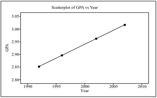
Graph: Construct a scatterplot using excel as follows:
Step 1: Enter the data in Excel.
Step 2: Select the data. Click on Insert
Step 3: Now, put the cursor on the graph and a plus sign appears on the right hand side.
Step 4: Click on the plus sign and check the box for trend line.
Hence, the obtained graph is shown below:
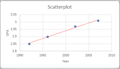
Interpretation: From the scatterplot, it can be seen that there is a linear dependency between GPA and year.
(c)
Section 1:
To find: The 95% confidence interval for the slope by hand.
(c)
Section 1:
Answer to Problem 30E
Solution: The confidence interval is
Explanation of Solution
Calculation: Now, compute
Year (x) |
GPA (y) |
|||
1992 |
2.85 |
2.852 |
0.000004 |
52.5625 |
1996 |
2.90 |
2.896 |
0.000016 |
10.5625 |
2002 |
2.97 |
2.962 |
0.000064 |
7.5625 |
2007 |
3.01 |
3.017 |
0.000049 |
60.0625 |
Now, compute the standard error of slope of regression
For 5% level of significance and
Compute the confidence interval as follows:
Interpretation: It can be said with 95% confidence that the GPA will increase between 0.008 and 0.014 over the time.
Section 2:
To find: The 95% confidence interval for the slope by software.
Section 2:
Answer to Problem 30E
Solution: The confidence interval is
Explanation of Solution
Calculation: Obtain the regression line using Excel as follows:
Step 1: Click on Data
Step 3: Enter Y variable and X variable input range.
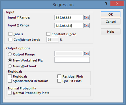
Step 4: Click ‘Ok’ to obtain the result.
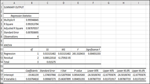
Hence, the obtained confidence interval for
Interpretation: Therefore, it can be concluded that the 95% confidence interval obtained by hand matched with the 95% confidence interval obtained by software.
Want to see more full solutions like this?
Chapter 10 Solutions
Introduction to the Practice of Statistics 9E & LaunchPad for Introduction to the Practice of Statistics 9E (Twelve-Month Access)


- ons 12. A sociologist hypothesizes that the crime rate is higher in areas with higher poverty rate and lower median income. She col- lects data on the crime rate (crimes per 100,000 residents), the poverty rate (in %), and the median income (in $1,000s) from 41 New England cities. A portion of the regression results is shown in the following table. Standard Coefficients error t stat p-value Intercept -301.62 549.71 -0.55 0.5864 Poverty 53.16 14.22 3.74 0.0006 Income 4.95 8.26 0.60 0.5526 a. b. Are the signs as expected on the slope coefficients? Predict the crime rate in an area with a poverty rate of 20% and a median income of $50,000. 3. Using data from 50 workarrow_forward2. The owner of several used-car dealerships believes that the selling price of a used car can best be predicted using the car's age. He uses data on the recent selling price (in $) and age of 20 used sedans to estimate Price = Po + B₁Age + ε. A portion of the regression results is shown in the accompanying table. Standard Coefficients Intercept 21187.94 Error 733.42 t Stat p-value 28.89 1.56E-16 Age -1208.25 128.95 -9.37 2.41E-08 a. What is the estimate for B₁? Interpret this value. b. What is the sample regression equation? C. Predict the selling price of a 5-year-old sedan.arrow_forwardian income of $50,000. erty rate of 13. Using data from 50 workers, a researcher estimates Wage = Bo+B,Education + B₂Experience + B3Age+e, where Wage is the hourly wage rate and Education, Experience, and Age are the years of higher education, the years of experience, and the age of the worker, respectively. A portion of the regression results is shown in the following table. ni ogolloo bash 1 Standard Coefficients error t stat p-value Intercept 7.87 4.09 1.93 0.0603 Education 1.44 0.34 4.24 0.0001 Experience 0.45 0.14 3.16 0.0028 Age -0.01 0.08 -0.14 0.8920 a. Interpret the estimated coefficients for Education and Experience. b. Predict the hourly wage rate for a 30-year-old worker with four years of higher education and three years of experience.arrow_forward
- 1. If a firm spends more on advertising, is it likely to increase sales? Data on annual sales (in $100,000s) and advertising expenditures (in $10,000s) were collected for 20 firms in order to estimate the model Sales = Po + B₁Advertising + ε. A portion of the regression results is shown in the accompanying table. Intercept Advertising Standard Coefficients Error t Stat p-value -7.42 1.46 -5.09 7.66E-05 0.42 0.05 8.70 7.26E-08 a. Interpret the estimated slope coefficient. b. What is the sample regression equation? C. Predict the sales for a firm that spends $500,000 annually on advertising.arrow_forwardCan you help me solve problem 38 with steps im stuck.arrow_forwardHow do the samples hold up to the efficiency test? What percentages of the samples pass or fail the test? What would be the likelihood of having the following specific number of efficiency test failures in the next 300 processors tested? 1 failures, 5 failures, 10 failures and 20 failures.arrow_forward
- The battery temperatures are a major concern for us. Can you analyze and describe the sample data? What are the average and median temperatures? How much variability is there in the temperatures? Is there anything that stands out? Our engineers’ assumption is that the temperature data is normally distributed. If that is the case, what would be the likelihood that the Safety Zone temperature will exceed 5.15 degrees? What is the probability that the Safety Zone temperature will be less than 4.65 degrees? What is the actual percentage of samples that exceed 5.25 degrees or are less than 4.75 degrees? Is the manufacturing process producing units with stable Safety Zone temperatures? Can you check if there are any apparent changes in the temperature pattern? Are there any outliers? A closer look at the Z-scores should help you in this regard.arrow_forwardNeed help pleasearrow_forwardPlease conduct a step by step of these statistical tests on separate sheets of Microsoft Excel. If the calculations in Microsoft Excel are incorrect, the null and alternative hypotheses, as well as the conclusions drawn from them, will be meaningless and will not receive any points. 4. One-Way ANOVA: Analyze the customer satisfaction scores across four different product categories to determine if there is a significant difference in means. (Hints: The null can be about maintaining status-quo or no difference among groups) H0 = H1=arrow_forward
- Please conduct a step by step of these statistical tests on separate sheets of Microsoft Excel. If the calculations in Microsoft Excel are incorrect, the null and alternative hypotheses, as well as the conclusions drawn from them, will be meaningless and will not receive any points 2. Two-Sample T-Test: Compare the average sales revenue of two different regions to determine if there is a significant difference. (Hints: The null can be about maintaining status-quo or no difference among groups; if alternative hypothesis is non-directional use the two-tailed p-value from excel file to make a decision about rejecting or not rejecting null) H0 = H1=arrow_forwardPlease conduct a step by step of these statistical tests on separate sheets of Microsoft Excel. If the calculations in Microsoft Excel are incorrect, the null and alternative hypotheses, as well as the conclusions drawn from them, will be meaningless and will not receive any points 3. Paired T-Test: A company implemented a training program to improve employee performance. To evaluate the effectiveness of the program, the company recorded the test scores of 25 employees before and after the training. Determine if the training program is effective in terms of scores of participants before and after the training. (Hints: The null can be about maintaining status-quo or no difference among groups; if alternative hypothesis is non-directional, use the two-tailed p-value from excel file to make a decision about rejecting or not rejecting the null) H0 = H1= Conclusion:arrow_forwardPlease conduct a step by step of these statistical tests on separate sheets of Microsoft Excel. If the calculations in Microsoft Excel are incorrect, the null and alternative hypotheses, as well as the conclusions drawn from them, will be meaningless and will not receive any points. The data for the following questions is provided in Microsoft Excel file on 4 separate sheets. Please conduct these statistical tests on separate sheets of Microsoft Excel. If the calculations in Microsoft Excel are incorrect, the null and alternative hypotheses, as well as the conclusions drawn from them, will be meaningless and will not receive any points. 1. One Sample T-Test: Determine whether the average satisfaction rating of customers for a product is significantly different from a hypothetical mean of 75. (Hints: The null can be about maintaining status-quo or no difference; If your alternative hypothesis is non-directional (e.g., μ≠75), you should use the two-tailed p-value from excel file to…arrow_forward
 MATLAB: An Introduction with ApplicationsStatisticsISBN:9781119256830Author:Amos GilatPublisher:John Wiley & Sons Inc
 Probability and Statistics for Engineering and th...StatisticsISBN:9781305251809Author:Jay L. DevorePublisher:Cengage Learning
 Statistics for The Behavioral Sciences (MindTap C...StatisticsISBN:9781305504912Author:Frederick J Gravetter, Larry B. WallnauPublisher:Cengage Learning
 Elementary Statistics: Picturing the World (7th E...StatisticsISBN:9780134683416Author:Ron Larson, Betsy FarberPublisher:PEARSON
 The Basic Practice of StatisticsStatisticsISBN:9781319042578Author:David S. Moore, William I. Notz, Michael A. FlignerPublisher:W. H. Freeman
 Introduction to the Practice of StatisticsStatisticsISBN:9781319013387Author:David S. Moore, George P. McCabe, Bruce A. CraigPublisher:W. H. Freeman