
Concept explainers
Videos
Stopping Distances
In a study on speed control, it was found that the main reasons for regulations were to make traffic flow more efficient and to minimize the risk of danger. An area that was focused on in the study was the distance required to completely stop a vehicle at various speeds. Use the following table to answer the questions.
| MPH | Braking distance (feet) |
| 20 30 40 50 60 80 |
20 45 81 133 205 411 |
Assume MPH is going to be used to predict stopping distance.
1. Which of the two variables is the independent variable?
2. Which is the dependent variable?
3. What type of variable is the independent variable?
4. What type of variable is the dependent variable?
5. Construct a
6. Is there a linear relationship between the two variables?
7. Redraw the scatter plot, and change the distances between the independent-variable numbers. Does the relationship look different?
8. Is the relationship positive or negative?
9. Can braking distance be accurately predicted from MPH?
10.List some other variables that affect braking distance.
11. Compute the value of r.
12. Is r significant at α = 0.05?
1.
To identify: The independent variable.
Answer to Problem 1AC
The independent variable is MPH (miles per hour).
Explanation of Solution
Given info:
The table shows the MPH (miles per hour) and Braking distance in feet.
Calculation:
Independent variable:
If the variable does not dependent on the other variables then the variables are said to be independent variable.
Here, the variable “Miles per hour” does not depend on the other variables. Thus, the independent variable is MPH (miles per hour).
2.
To identify: The dependent variable.
Answer to Problem 1AC
The dependent variable is Braking distance (feet).
Explanation of Solution
Calculation:
Dependent variable:
If the variable depends on the other variables then the variable is said to be dependent variable.
Here, the variable “Braking distance” depends on the other variables. That is the variable braking distance depends on the MPH (miles per hour). Thus, the dependent variable is Braking distance (feet).
3.
The type of variable is the independent variable.
Answer to Problem 1AC
The type of independent variable is the continuous quantitative variable.
Explanation of Solution
Justification:
Continuous quantitative variable:
If the variable takes values on interval scale then the variable is said to be continuous quantitative variable. In the continuous variable, the infinitely many number of values can be considered.
Here, the independent variable miles per hour (MPH) can take any value from a wide range of values. Thus, the independent variable miles per hour (MPH) is continuous quantitative variable.
4.
The type of variable is the dependent variable.
Answer to Problem 1AC
The type of dependent variable is the continuous quantitative variable.
Explanation of Solution
Justification:
Here, the dependent variable braking distance (feet) can take any value from a wide range of values. Thus, the independent variable braking distance (feet) is continuous quantitative variable.
5.
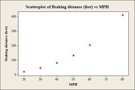
To construct: The scatterplot for the data.
Answer to Problem 1AC
The scatterplot for the data given data using Minitab software is:
Explanation of Solution
Calculation:
The data shows the MPH (miles per hour) and Braking distance (feet) for vehicles.
Step by step procedure to obtain scatterplot using the MINITAB software:
- Choose Graph > Scatterplot.
- Choose Simple and then click OK.
- Under Y variables, enter a column of Braking distance (feet).
- Under X variables, enter a column of MPH.
- Click OK.
6.
To check: Whether there is a linear relationship between the two variables.
Answer to Problem 1AC
Yes, there is a linear relationship between the two variables.
Explanation of Solution
Justification:
The horizontal axis represents miles per hour (MPH) and vertical axis represents braking distance (feet).
From the plot, it is observed that there is a linear relationship between the variables miles per hour (MPH) and braking distance (feet) because the data points show a distinct pattern.
7.
To construct: The scatterplot for the changed data.
To check: Whether the relationship looks different or not.
Answer to Problem 1AC
The scatterplot for the changed data by using Minitab software is:
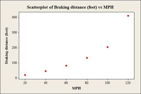
The increments will change the appearance of the relationship if changing the distance between the independent-variable (mph).
Explanation of Solution
Calculation:
The data shows the MPH (miles per hour) and Braking distance (feet) for vehicles.
After changing the distance between the independent-variable numbers, the number of the independent-variable is, 20, 40, 60, 80, 100 and 120.
Step by step procedure to obtain scatterplot using the MINITAB software:
- Choose Graph > Scatterplot.
- Choose Simple and then click OK.
- Under Y variables, enter a column of Braking distance (feet).
- Under X variables, enter a column of MPH.
- Click OK.
Justification:
From the graphs it can be observed that, after changing the distance between the independent-variable (mph), the increments will change the appearance of the relationship.
8.
To check: Whether the relationship is positive or negative.
Answer to Problem 1AC
The relationship is positive.
Explanation of Solution
Justification:
The relationship is positive because the values of independent variable increases then the values of corresponding dependent variable are increases.
9.
To check: Whether the braking distance can be accurately predicted from MPH.
Answer to Problem 1AC
Yes, the braking distance can be accurately predicted from MPH.
Explanation of Solution
Justification:
Here, the braking distance can be accurately predicted from MPH because the relationship between two variables MPH and Breaking distance is strong.
10.
To list: The other variables that affect braking distance.
Answer to Problem 1AC
The other variables that affect braking distance are road conditions, driver response time and condition of the brakes.
Explanation of Solution
Justification:
Answer may wary. One of the possible answers is as follows.
The variable affecting the braking distance are road conditions, driver response time and condition of the brakes.
11.
To compute: The value of r.
Answer to Problem 1AC
The value of r is 0.966.
Explanation of Solution
Calculation:
Correlation coefficient r:
Software Procedure:
Step-by-step procedure to obtain the ‘correlation coefficient’ using the MINITAB software:
- Select Stat > Basic Statistics > Correlation.
- In Variables, select MPH and Braking distance (feet) from the box on the left.
- Click OK.
Output using the MINITAB software is given below:
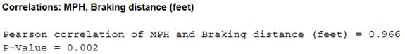
Thus, the Pearson correlation of MPH and Braking distance is 0.966.
12.
To check: Whether or not the r value is significant at 0.05.
Answer to Problem 1AC
Yes, the r value is significant at 0.05.
Explanation of Solution
Calculation:
Here, the r value is significant is checked. So, the claim is that the r value is significant.
The hypotheses are given below:
Null hypothesis:
That is, there is no linear relation between the MPH and Braking distance.
Alternative hypothesis:
That is, there is linear relation between the MPH and Braking distance.
The sample size is 6.
The formula to find the degrees of the freedom is
That is,
From the “TABLE –I: Critical Values for the PPMC”, the critical value for 4 degrees of freedom and
Rejection Rule:
If the absolute value of r is greater than the critical value then reject the null hypothesis.
Conclusion:
From part (11), the Pearson correlation of MPH and Braking distance is 0.966. That is the absolute value of r is 0.966.
Here,
By the rejection rule, reject the null hypothesis.
There is sufficient evidence to support the claim that “there is a linear relation between the MPH and Braking distance”.
Want to see more full solutions like this?
Chapter 10 Solutions
Elementary Statistics: A Step By Step Approach
Additional Math Textbook Solutions
Introductory Statistics
Elementary & Intermediate Algebra
A First Course in Probability (10th Edition)
Calculus: Early Transcendentals (2nd Edition)
Elementary Statistics: Picturing the World (7th Edition)
Basic College Mathematics


- A company found that the daily sales revenue of its flagship product follows a normal distribution with a mean of $4500 and a standard deviation of $450. The company defines a "high-sales day" that is, any day with sales exceeding $4800. please provide a step by step on how to get the answers in excel Q: What percentage of days can the company expect to have "high-sales days" or sales greater than $4800? Q: What is the sales revenue threshold for the bottom 10% of days? (please note that 10% refers to the probability/area under bell curve towards the lower tail of bell curve) Provide answers in the yellow cellsarrow_forwardFind the critical value for a left-tailed test using the F distribution with a 0.025, degrees of freedom in the numerator=12, and degrees of freedom in the denominator = 50. A portion of the table of critical values of the F-distribution is provided. Click the icon to view the partial table of critical values of the F-distribution. What is the critical value? (Round to two decimal places as needed.)arrow_forwardA retail store manager claims that the average daily sales of the store are $1,500. You aim to test whether the actual average daily sales differ significantly from this claimed value. You can provide your answer by inserting a text box and the answer must include: Null hypothesis, Alternative hypothesis, Show answer (output table/summary table), and Conclusion based on the P value. Showing the calculation is a must. If calculation is missing,so please provide a step by step on the answers Numerical answers in the yellow cellsarrow_forward
 Glencoe Algebra 1, Student Edition, 9780079039897...AlgebraISBN:9780079039897Author:CarterPublisher:McGraw Hill
 Functions and Change: A Modeling Approach to Coll...AlgebraISBN:9781337111348Author:Bruce Crauder, Benny Evans, Alan NoellPublisher:Cengage Learning
 Big Ideas Math A Bridge To Success Algebra 1: Stu...AlgebraISBN:9781680331141Author:HOUGHTON MIFFLIN HARCOURTPublisher:Houghton Mifflin Harcourt
 Holt Mcdougal Larson Pre-algebra: Student Edition...AlgebraISBN:9780547587776Author:HOLT MCDOUGALPublisher:HOLT MCDOUGAL
 College AlgebraAlgebraISBN:9781305115545Author:James Stewart, Lothar Redlin, Saleem WatsonPublisher:Cengage Learning
 Algebra and Trigonometry (MindTap Course List)AlgebraISBN:9781305071742Author:James Stewart, Lothar Redlin, Saleem WatsonPublisher:Cengage Learning