Concept explainers
To determine: The difference shown by the second set of sample from the first one.
Introduction
Company TT is a division of company DM. It was about to launch a new product. Ms. MY, the
Table 1
| Sample | Mean | Range |
| 1 | 45.01 | 0.85 |
| 2 | 44.99 | 0.89 |
| 3 | 45.02 | 0.86 |
| 4 | 45 | 0.91 |
| 5 | 45.04 | 0.87 |
| 6 | 44.98 | 0.9 |
| 7 | 44.91 | 0.86 |
| 8 | 45.04 | 0.89 |
| 9 | 45 | 0.85 |
| 10 | 44.97 | 0.91 |
| 11 | 45.11 | 0.84 |
| 12 | 44.96 | 0.87 |
| 13 | 45 | 0.86 |
| 14 | 44.92 | 0.89 |
| 15 | 45.06 | 0.87 |
| 16 | 44.94 | 0.86 |
| 17 | 45 | 0.85 |
| 18 | 45.03 | 0.88 |
Quiet disappointed with the end results, the manager was figuring out ways to improve the process and free the capital expenditure of $10,000. A former professor suggested going for more samples with less sample sizes. JM conducted the analysis on 27 samples of 5 observations each and the results are tabulated below:
Table 2
| Sample | Mean | Range |
| 1 | 44.96 | 0.42 |
| 2 | 44.98 | 0.39 |
| 3 | 44.96 | 0.41 |
| 4 | 44.97 | 0.37 |
| 5 | 45.02 | 0.39 |
| 6 | 45.03 | 0.4 |
| 7 | 45.04 | 0.39 |
| 8 | 45.02 | 0.42 |
| 9 | 45.08 | 0.38 |
| 10 | 45.12 | 0.4 |
| 11 | 45.07 | 0.41 |
| 12 | 45.02 | 0.38 |
| 13 | 45.01 | 0.41 |
| 14 | 44.98 | 0.4 |
| 15 | 45 | 0.39 |
| 16 | 44.95 | 0.41 |
| 17 | 44.94 | 0.43 |
| 18 | 44.94 | 0.4 |
| 19 | 44.87 | 0.38 |
| 20 | 44.95 | 0.41 |
| 21 | 44.93 | 0.39 |
| 22 | 44.96 | 0.41 |
| 23 | 44.99 | 0.4 |
| 24 | 45 | 0.44 |
| 25 | 45.03 | 0.42 |
| 26 | 45.04 | 0.38 |
| 27 | 45.03 | 0.4 |
Answer to Problem 2.2CQ
Explanation of Solution
Given information:
Table 3
| Sample | Mean | Range |
| 1 | 45.01 | 0.85 |
| 2 | 44.99 | 0.89 |
| 3 | 45.02 | 0.86 |
| 4 | 45 | 0.91 |
| 5 | 45.04 | 0.87 |
| 6 | 44.98 | 0.9 |
| 7 | 44.91 | 0.86 |
| 8 | 45.04 | 0.89 |
| 9 | 45 | 0.85 |
| 10 | 44.97 | 0.91 |
| 11 | 45.11 | 0.84 |
| 12 | 44.96 | 0.87 |
| 13 | 45 | 0.86 |
| 14 | 44.92 | 0.89 |
| 15 | 45.06 | 0.87 |
| 16 | 44.94 | 0.86 |
| 17 | 45 | 0.85 |
| 18 | 45.03 | 0.88 |
Formula:
Mean Chart:
Difference shown by the second set of sample from the first one:
Date set:1
Table 4
| Sample | Mean | Range |
| 1 | 45.01 | 0.85 |
| 2 | 44.99 | 0.89 |
| 3 | 45.02 | 0.86 |
| 4 | 45 | 0.91 |
| 5 | 45.04 | 0.87 |
| 6 | 44.98 | 0.9 |
| 7 | 44.91 | 0.86 |
| 8 | 45.04 | 0.89 |
| 9 | 45 | 0.85 |
| 10 | 44.97 | 0.91 |
| 11 | 45.11 | 0.84 |
| 12 | 44.96 | 0.87 |
| 13 | 45 | 0.86 |
| 14 | 44.92 | 0.89 |
| 15 | 45.06 | 0.87 |
| 16 | 44.94 | 0.86 |
| 17 | 45 | 0.85 |
| 18 | 45.03 | 0.88 |
| 45 | 0.872777778 |
Excel worksheet:
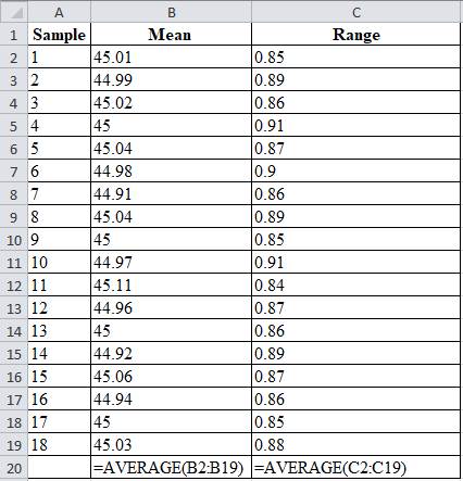
From factors of three-sigma chart, for n=20, A2 = 0.18; D3 = 0.41; D4 = 1.59
Mean control chart:
Range control chart:
Upper control limit:
The upper control limit is calculated by adding the product of 0.18 and 0.873 with 45, which yields 45.156.
Lower control limit:
The lower control limit is calculated by subtracting the product of 0.18 and 0.873 with 45, which yields 44.842.
A graph is plotted using the UCL, LCL and samples values.
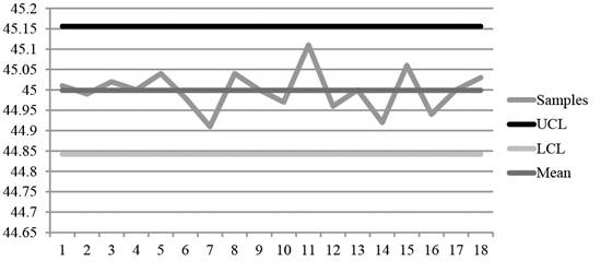
Diagram 1
Date set: 2
Table 5
| Sample | Mean | Range |
| 1 | 44.96 | 0.42 |
| 2 | 44.98 | 0.39 |
| 3 | 44.96 | 0.41 |
| 4 | 44.97 | 0.37 |
| 5 | 45.02 | 0.39 |
| 6 | 45.03 | 0.4 |
| 7 | 45.04 | 0.39 |
| 8 | 45.02 | 0.42 |
| 9 | 45.08 | 0.38 |
| 10 | 45.12 | 0.4 |
| 11 | 45.07 | 0.41 |
| 12 | 45.02 | 0.38 |
| 13 | 45.01 | 0.41 |
| 14 | 44.98 | 0.4 |
| 15 | 45 | 0.39 |
| 16 | 44.95 | 0.41 |
| 17 | 44.94 | 0.43 |
| 18 | 44.94 | 0.4 |
| 19 | 44.87 | 0.38 |
| 20 | 44.95 | 0.41 |
| 21 | 44.93 | 0.39 |
| 22 | 44.96 | 0.41 |
| 23 | 44.99 | 0.4 |
| 24 | 45 | 0.44 |
| 25 | 45.03 | 0.42 |
| 26 | 45.04 | 0.38 |
| 27 | 45.03 | 0.4 |
| 44.9959 | 0.40111 |
Excel worksheet:
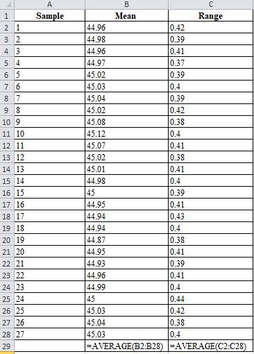
From factors of three-sigma chart, for n=20, A2 = 0.58
Mean control chart:
Range control chart:
Upper control limit:
The upper control limit is calculated by adding the product of 0.58 and 0.401 with 44.99, which yields 45.229.
Lower control limit:
The lower control limit is calculated by subtracting the product of 0.58 and 0.401 with 44.99, which yields 44.763.
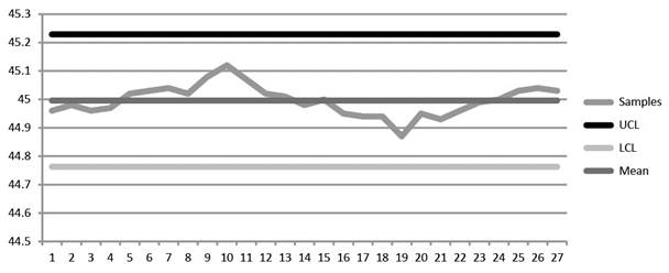
Diagram 2
On comparing Diagrams 1 and 2, it is evident that the second set of data has closer range of changes while the first set of data is scattered and reveals no information about the changes in the process.
Hence, the second sample reveals the changes in the process changes more clearly than the first set of data.
Want to see more full solutions like this?
Chapter 10 Solutions
Loose Leaf for Operations Management (The Mcgraw-hill Series in Operations and Decision Sciences)


- Employee In-Service Training ASSIGNMENT: In-Service Training. The intern is required to plan and implement two in-service training sessions for employees. Each in-service should last at least 10 but not more than 30 minutes and should be given to all employees affected. The preceptor or supervisor/unit manager must approve all in-service topics. 1) One presentation should be related to a policy or procedure of any kind (e.g. proper use of equipment); 2) The second presentation must be related to sanitation or safety. For each in-service presentation, the intern must develop a written class plan and a visual aid (may be a handout, poster, PowerPoint slide presentation, etc.) appropriate to the life experiences, cultural diversity and educational background of the target audience. The intern must also measure behavior change. Note, this cannot be measured by a written pre- and post- test. That would be measuring knowledge. The intern mustactually observe and document that the learners…arrow_forwardFor a dietary manager in a nursing home to train a dietary aidearrow_forwardDietary Management in a Nursing Home. As detailed as possible.arrow_forward
- For dietary management in a nursing home. As detailed as possible.arrow_forwardA small furniture manufacturer produces tables and chairs. Each product must go through three stages of the manufacturing process – assembly, finishing, and inspection. Each table requires 3 hours of assembly, 2 hours of finishing, and 1 hour of inspection. The profit per table is $120 while the profit per chair is $80. Currently, each week there are 200 hours of assembly time available, 180 hours of finishing time, and 40 hours of inspection time. Linear programming is to be used to develop a production schedule. Define the variables as follows: T = number of tables produced each week C= number of chairs produced each week According to the above information, what would the objective function be? (a) Maximize T+C (b) Maximize 120T + 80C (c) Maximize 200T+200C (d) Minimize 6T+5C (e) none of the above According to the information provided in Question 17, which of the following would be a necessary constraint in the problem? (a) T+C ≤ 40 (b) T+C ≤ 200 (c) T+C ≤ 180 (d) 120T+80C ≥ 1000…arrow_forwardAs much detail as possible. Dietary Management- Nursing Home Don't add any fill-in-the-blanksarrow_forward
- Menu Planning Instructions Use the following questions and points as a guide to completing this assignment. The report should be typed. Give a copy to the facility preceptor. Submit a copy in your Foodservice System Management weekly submission. 1. Are there any federal regulations and state statutes or rules with which they must comply? Ask preceptor about regulations that could prescribe a certain amount of food that must be kept on hand for emergencies, etc. Is the facility accredited by any agency such as Joint Commission? 2. Describe the kind of menu the facility uses (may include standard select menu, menu specific to station, non-select, select, room service, etc.) 3. What type of foodservice does the facility have? This could be various stations to choose from, self-serve, 4. conventional, cook-chill, assembly-serve, etc. Are there things about the facility or system that place a constraint on the menu to be served? Consider how patients/guests are served (e.g. do they serve…arrow_forwardWork with the chef and/or production manager to identify a menu item (or potential menu item) for which a standardized recipe is needed. Record the recipe with which you started and expand it to meet the number of servings required by the facility. Develop an evaluation rubric. Conduct an evaluation of the product. There should be three or more people evaluating the product for quality. Write a brief report of this activity • Product chosen and the reason why it was selected When and where the facility could use the product The standardized recipe sheet or card 。 o Use the facility's format or Design one of your own using a form of your choice; be sure to include the required elements • • Recipe title Yield and portion size Cooking time and temperature Ingredients and quantities Specify AP or EP Procedures (direction)arrow_forwardASSIGNMENT: Inventory, Answer the following questions 1. How does the facility survey inventory? 2. Is there a perpetual system in place? 3. How often do they do a physical inventory? 4. Participate in taking inventory. 5. Which type of stock system does the facility use? A. Minimum stock- includes a safety factor for replenishing stock B. Maximum stock- equal to a safety stock plus estimated usage (past usage and forecasts) C. Mini-max-stock allowed to deplete to a safety level before a new order is submitted to bring up inventory up to max again D. Par stock-stock brought up to the par level each time an order is placed regardless of the amount on hand at the time of order E. Other-(describe) Choose an appropriate product and determine how much of an item should be ordered. Remember the formula is: Demand during lead time + safety stock = amount to order Cost out an inventory according to data supplied. Remember that to do this, you will need to take an inventory, and will need to…arrow_forward
 Practical Management ScienceOperations ManagementISBN:9781337406659Author:WINSTON, Wayne L.Publisher:Cengage,
 Foundations of Business (MindTap Course List)MarketingISBN:9781337386920Author:William M. Pride, Robert J. Hughes, Jack R. KapoorPublisher:Cengage Learning
 Foundations of Business - Standalone book (MindTa...MarketingISBN:9781285193946Author:William M. Pride, Robert J. Hughes, Jack R. KapoorPublisher:Cengage Learning