Chapter 10, Problem 10.1.7RE

a.

To determine

To construct: The scatterplot for the give data.

Answer to Problem 10.1.7RE

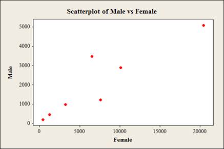
The scatterplot for the data is as follows,

Explanation of Solution

Given info:

The data represents the numbers of male and female physicians.

Calculation:

Software procedure:

Step by step procedure to obtain scatterplot using the MINITAB software:

• Choose Graph > Scatterplot.
• Choose Simple and then click OK.
• Under Y variables, enter a column of Male.
• Under X variables, enter a column of Female.
• Click OK.

b.

To determine

To compute: The value of the correlation coefficient.

Answer to Problem 10.1.7RE

The value of the correlation coefficient is 0.907.

Explanation of Solution

Calculation:

Correlation coefficient r:

Software Procedure:

Step-by-step procedure to obtain the ‘correlation coefficient’ using the MINITAB software:

• Select Stat >Basic Statistics > Correlation.
• In Variables, select Male and Female from the box on the left.
• Click OK.

Output using the MINITAB software is given below:

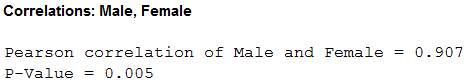
Thus, the value of the correlation is 0.907.

c.

To determine

To test: The significance of the correlation coefficient at $\alpha =0.01$ using Table I.

Answer to Problem 10.1.7RE

The conclusion is that, there is linear relation between the number of male and female physicians.

Explanation of Solution

Given info:

The level of significance is $\alpha =0.01$ and the sample size is 7.

Calculation:

The hypotheses are given below:

Null hypothesis:

$H_0:\rho =0$

That is, there is no linear relation between the number of male physicians and number of female physicians.

Alternative hypothesis:

$H_1:\rho \ne 0$

That is, there is a linear relation between the number of male physicians and number of female physicians.

The formula to obtain the degrees of the freedom is $n-2$.

That is,

$\begin{array}{c}n-2=7-2\\ =5\end{array}$

From the “TABLE –I: Critical Values for the PPMC”, the critical value for 5 degrees of freedom and $\alpha =0.01$ level of significance is 0.875.

Rejection Rule:

If the absolute value of r is greater than the critical value then reject the null hypothesis.

Conclusion:

From part (b), the value of the correlation of Men and Women is 0.907. That is the absolute value of r is 0.907.

Here, the absolute value of r is greater than the critical value.

That is, $\left|r\right|\left(=0.907\right)<\text{critical value}\left(=0.875\right)$.

By the rejection rule, the null hypothesis is rejected.

Therefore, there is sufficient evidence to support the claim that “there is a linear relation between the number of male and female physicians”.

d.

To determine

To find: The regression equation for the given data

Answer to Problem 10.1.7RE

The regression equation for the given data is $\widehat{y}=103+3.41x$.

Explanation of Solution

Calculation:

Regression:

Software procedure:

Step by step procedure to obtain the regression equation using the MINITAB software:

• Choose Stat > Regression > Regression.
• In Responses, enter the column of Female.
• In Predictors, enter the column of Male.
• Click OK.

Output using the MINITAB software is given below:

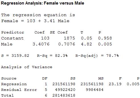
Thus, the regression equation for the given data is $\widehat{y}=103+3.41x$.

e.

To determine

To construct: The regression line on the scatter plot if appropriate.

Answer to Problem 10.1.7RE

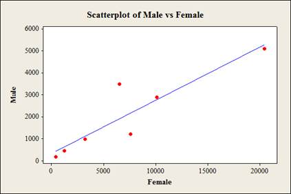
The regression line on the scatter plot the scatterplot is as follows,

Explanation of Solution

Calculation:

Step by step procedure to obtain scatterplot using the MINITAB software:

• Choose Graph > Scatterplot.
• Choose With Regression and then click OK.
• Under Y variables, enter a column of Male.
• Under X variables, enter a column of Female.
• Click OK.

f.

To determine

To predict: The number of male specialists when there are 2,000 female specialists.

Answer to Problem 10.1.7RE

The predicted value of number of male specialists when there are 2,000 female specialists is 6,923.

Explanation of Solution

From part (d), the regression equation for the given data is $\widehat{y}=103+3.41x$.

Substitute x as 2,000 in the regression equation

$\begin{array}{c}\widehat{y}=103+3.41x\\ =103+\left(3.41\times 2,000\right)\\ =103+6,820\\ =6,923\end{array}$

Thus, the predicted value of number of male specialists when there are 2,000 female specialists is 6,923.