
Concept explainers
Videos
a.
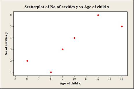
To construct: The
a.
Answer to Problem 20CQ
Output using the MINITAB software is given below:
Explanation of Solution
Given info:
The data shows the age of a child (x) and the number of cavities (y) values.
Calculation:
Step by step procedure to obtain scatterplot using the MINITAB software:
- Choose Graph > Scatterplot.
- Choose Simple and then click OK.
- Under Y variables, enter a column ofNo.of cavities.
- Under X variables, enter a column ofAge of child.
- Click OK.
b.
To compute: The value of the
b.
Answer to Problem 20CQ
The value of the
Explanation of Solution
Calculation:
Correlation coefficient r:
Software Procedure:
Step-by-step procedure to obtain the ‘correlation coefficient’ using the MINITAB software:
- Select Stat >Basic Statistics > Correlation.
- In Variables, select x and y from the box on the left.
- Click OK.
Output using the MINITAB software is given below:
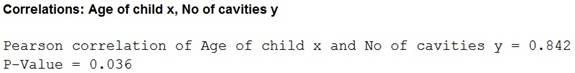
From the MINITAB output, the value of the correlation is 0.842.
c.
To test: The significance of the correlation coefficient at
c.
Answer to Problem 20CQ
The conclusion is that,there is a linear relation between the age of a child and the number of cavities.
Explanation of Solution
Given info:
The level of significance is
Calculation:
The hypotheses are given below:
Null hypothesis:
That is, there is no linear relation betweenthe age of a child and the number of cavities.
Alternative hypothesis:
That is, there is a linear relation between the age of a child and the number of cavities.
The sample size is 6.
The formula to find the degrees of the freedom is
That is,
From the “TABLE –I: Critical Values for the PPMC”, the critical value for 4 degrees of freedom and
Rejection Rule:
If the absolute value of r is greater than the critical value then reject the null hypothesis.
Conclusion:
From part (b), the value of r is0.842that is the absolute value of r is 0.842.
Here, the absolute value of r is greater than the critical value
That is,
By the rejection rule,reject the null hypothesis.
There is asufficient evidence to support the claim that “there is alinear relation betweenthe age of a child and the number of cavities”.
d.
To find: The regression equation for the given data.
d.
Answer to Problem 20CQ
The regression equation for the given datais
Explanation of Solution
Calculation:
Regression:
Software procedure:
Step by step procedure to obtain the regression equation using the MINITAB software:
- Choose Stat > Regression > Regression.
- In Responses, enter the column ofNo.of cavities.
- In Predictors, enter the column ofAge of child.
- Click OK.
Output using the MINITAB software is given below:
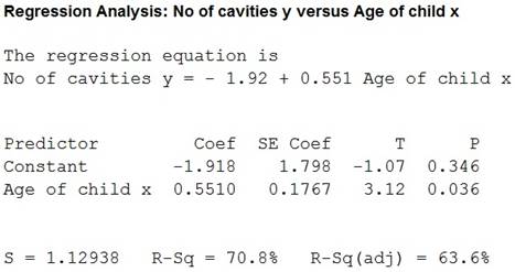
Thus, regression equation for the given datais
e.
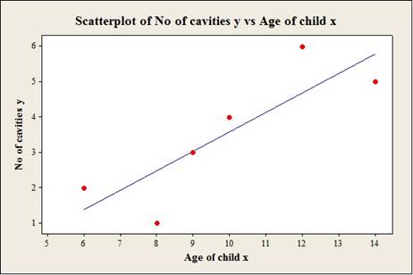
To construct: The scatterplot for the variablesthe age of a child and the number of cavitieswith regression line.
e.
Answer to Problem 20CQ
Output using the MINITAB software is given below:
Explanation of Solution
Calculation:
Step by step procedure to obtain scatterplot using the MINITAB software:
- Choose Graph > Scatterplot.
- Choose with line and then click OK.
- Under Y variables, enter a column of No.of cavities.
- Under X variables, enter a column ofAge of child.
- Click OK.
f.
To obtain: The predicted value of the number of cavities for a child of 11.
f.
Answer to Problem 20CQ
Thepredicted value of the number of cavities is 4.143.
Explanation of Solution
Calculation:
Thus, regression equation for the given datais
Substitute x as 11 in the regression equation
Thus, the predicted value of the number of cavities is 4.143.
Want to see more full solutions like this?
Chapter 10 Solutions
ELEMENTARY STATISTICS W/CONNECT >IP<


- I just need to know why this is wrong below: What is the test statistic W? W=5 (incorrect) and What is the p-value of this test? (p-value < 0.001-- incorrect) Use the Wilcoxon signed rank test to test the hypothesis that the median number of pages in the statistics books in the library from which the sample was taken is 400. A sample of 12 statistics books have the following numbers of pages pages 127 217 486 132 397 297 396 327 292 256 358 272 What is the sum of the negative ranks (W-)? 75 What is the sum of the positive ranks (W+)? 5What type of test is this? two tailedWhat is the test statistic W? 5 These are the critical values for a 1-tailed Wilcoxon Signed Rank test for n=12 Alpha Level 0.001 0.005 0.01 0.025 0.05 0.1 0.2 Critical Value 75 70 68 64 60 56 50 What is the p-value for this test? p-value < 0.001arrow_forwardons 12. A sociologist hypothesizes that the crime rate is higher in areas with higher poverty rate and lower median income. She col- lects data on the crime rate (crimes per 100,000 residents), the poverty rate (in %), and the median income (in $1,000s) from 41 New England cities. A portion of the regression results is shown in the following table. Standard Coefficients error t stat p-value Intercept -301.62 549.71 -0.55 0.5864 Poverty 53.16 14.22 3.74 0.0006 Income 4.95 8.26 0.60 0.5526 a. b. Are the signs as expected on the slope coefficients? Predict the crime rate in an area with a poverty rate of 20% and a median income of $50,000. 3. Using data from 50 workarrow_forward2. The owner of several used-car dealerships believes that the selling price of a used car can best be predicted using the car's age. He uses data on the recent selling price (in $) and age of 20 used sedans to estimate Price = Po + B₁Age + ε. A portion of the regression results is shown in the accompanying table. Standard Coefficients Intercept 21187.94 Error 733.42 t Stat p-value 28.89 1.56E-16 Age -1208.25 128.95 -9.37 2.41E-08 a. What is the estimate for B₁? Interpret this value. b. What is the sample regression equation? C. Predict the selling price of a 5-year-old sedan.arrow_forward
- ian income of $50,000. erty rate of 13. Using data from 50 workers, a researcher estimates Wage = Bo+B,Education + B₂Experience + B3Age+e, where Wage is the hourly wage rate and Education, Experience, and Age are the years of higher education, the years of experience, and the age of the worker, respectively. A portion of the regression results is shown in the following table. ni ogolloo bash 1 Standard Coefficients error t stat p-value Intercept 7.87 4.09 1.93 0.0603 Education 1.44 0.34 4.24 0.0001 Experience 0.45 0.14 3.16 0.0028 Age -0.01 0.08 -0.14 0.8920 a. Interpret the estimated coefficients for Education and Experience. b. Predict the hourly wage rate for a 30-year-old worker with four years of higher education and three years of experience.arrow_forward1. If a firm spends more on advertising, is it likely to increase sales? Data on annual sales (in $100,000s) and advertising expenditures (in $10,000s) were collected for 20 firms in order to estimate the model Sales = Po + B₁Advertising + ε. A portion of the regression results is shown in the accompanying table. Intercept Advertising Standard Coefficients Error t Stat p-value -7.42 1.46 -5.09 7.66E-05 0.42 0.05 8.70 7.26E-08 a. Interpret the estimated slope coefficient. b. What is the sample regression equation? C. Predict the sales for a firm that spends $500,000 annually on advertising.arrow_forwardCan you help me solve problem 38 with steps im stuck.arrow_forward
- How do the samples hold up to the efficiency test? What percentages of the samples pass or fail the test? What would be the likelihood of having the following specific number of efficiency test failures in the next 300 processors tested? 1 failures, 5 failures, 10 failures and 20 failures.arrow_forwardThe battery temperatures are a major concern for us. Can you analyze and describe the sample data? What are the average and median temperatures? How much variability is there in the temperatures? Is there anything that stands out? Our engineers’ assumption is that the temperature data is normally distributed. If that is the case, what would be the likelihood that the Safety Zone temperature will exceed 5.15 degrees? What is the probability that the Safety Zone temperature will be less than 4.65 degrees? What is the actual percentage of samples that exceed 5.25 degrees or are less than 4.75 degrees? Is the manufacturing process producing units with stable Safety Zone temperatures? Can you check if there are any apparent changes in the temperature pattern? Are there any outliers? A closer look at the Z-scores should help you in this regard.arrow_forwardNeed help pleasearrow_forward
- Please conduct a step by step of these statistical tests on separate sheets of Microsoft Excel. If the calculations in Microsoft Excel are incorrect, the null and alternative hypotheses, as well as the conclusions drawn from them, will be meaningless and will not receive any points. 4. One-Way ANOVA: Analyze the customer satisfaction scores across four different product categories to determine if there is a significant difference in means. (Hints: The null can be about maintaining status-quo or no difference among groups) H0 = H1=arrow_forwardPlease conduct a step by step of these statistical tests on separate sheets of Microsoft Excel. If the calculations in Microsoft Excel are incorrect, the null and alternative hypotheses, as well as the conclusions drawn from them, will be meaningless and will not receive any points 2. Two-Sample T-Test: Compare the average sales revenue of two different regions to determine if there is a significant difference. (Hints: The null can be about maintaining status-quo or no difference among groups; if alternative hypothesis is non-directional use the two-tailed p-value from excel file to make a decision about rejecting or not rejecting null) H0 = H1=arrow_forwardPlease conduct a step by step of these statistical tests on separate sheets of Microsoft Excel. If the calculations in Microsoft Excel are incorrect, the null and alternative hypotheses, as well as the conclusions drawn from them, will be meaningless and will not receive any points 3. Paired T-Test: A company implemented a training program to improve employee performance. To evaluate the effectiveness of the program, the company recorded the test scores of 25 employees before and after the training. Determine if the training program is effective in terms of scores of participants before and after the training. (Hints: The null can be about maintaining status-quo or no difference among groups; if alternative hypothesis is non-directional, use the two-tailed p-value from excel file to make a decision about rejecting or not rejecting the null) H0 = H1= Conclusion:arrow_forward
 Glencoe Algebra 1, Student Edition, 9780079039897...AlgebraISBN:9780079039897Author:CarterPublisher:McGraw Hill
 Functions and Change: A Modeling Approach to Coll...AlgebraISBN:9781337111348Author:Bruce Crauder, Benny Evans, Alan NoellPublisher:Cengage Learning
 Big Ideas Math A Bridge To Success Algebra 1: Stu...AlgebraISBN:9781680331141Author:HOUGHTON MIFFLIN HARCOURTPublisher:Houghton Mifflin Harcourt
 College AlgebraAlgebraISBN:9781305115545Author:James Stewart, Lothar Redlin, Saleem WatsonPublisher:Cengage Learning
 Algebra & Trigonometry with Analytic GeometryAlgebraISBN:9781133382119Author:SwokowskiPublisher:Cengage
 Algebra and Trigonometry (MindTap Course List)AlgebraISBN:9781305071742Author:James Stewart, Lothar Redlin, Saleem WatsonPublisher:Cengage Learning