
Videos
The article “Hydrogeochemical Characteristics of Groundwater in a Mid-Western Coastal Aquifer System” (S. Jeen. J. Kim, et al., Geosciences Journal, 2001:339–348) presents measurements of various properties of shallow groundwater in a certain aquifer system in Korea. Following are measurements of electrical conductivity (in microsiemens per centimeter) for 23 water samples.
2099 528 2030 1350 1018 384 1499
1265 375 424 789 810 522 513
488 200 215 486 257 557 260
461 500
- a. Find the mean.
- b. Find the standard deviation.
- c. Find the
median . - d. Construct a dotplot.
- e. Find the 10% trimmed mean.
- f. Find the first
quartile . - g. Find the third quartile.
- h. Find the
interquartile range . - i. Construct a boxplot.
- j. Which of the points, if any, are outliers?
- k. If a histogram were constructed, would it be skewed to the left, skewed to the right, or approximately symmetric?
a.
Find the mean.
Answer to Problem 16SE
The mean is 740.0.
Explanation of Solution
Given info:
The data shows that the measurements of the electrical conductivity.
Calculation:
Step by step procedure for finding the mean concentration using Minitab software is follows:
- Choose Stat > Basic Statistics > Display Descriptive Statistics.
- In Variables enter the columns Measurements.
- Choose option statistics, and select Mean.
- Click OK.
Output using Minitab software is,
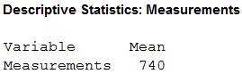
From the output the mean is 74.0.
b.
Find the standard deviation.
Answer to Problem 16SE
The standard deviation is 550.
Explanation of Solution
Calculation:
Step by step procedure for finding the mean concentration using Minitab software is follows:
- Choose Stat > Basic Statistics > Display Descriptive Statistics.
- In Variables enter the columns Measurements.
- Choose option statistics, and select Standard deviation.
- Click OK.
Output using Minitab software is,
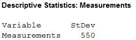
From the output the standard deviation is 550.
c.
Compute the median.
Answer to Problem 16SE
The median is 513.
Explanation of Solution
Calculation:
Step by step procedure for finding the median concentration is follows:
- Choose Stat > Basic Statistics > Display Descriptive Statistics.
- In Variables enter the columns Measurements.
- Choose option statistics, and select Median.
- Click OK.
Output using Minitab software is,
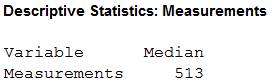
From the output the median is 513.
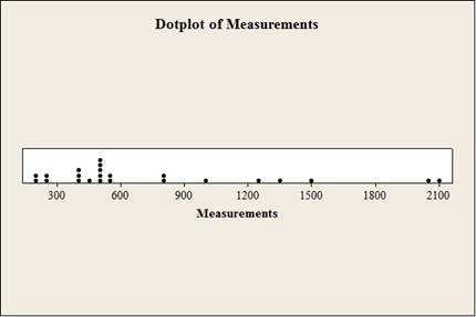
d.
Construct a dotplot.
Answer to Problem 16SE
The dotplot is,
Explanation of Solution
Calculation:
Step by step procedure to constructing dotplot using Minitab procedure is follows:
- Choose Graph > Dotplot.
- Choose One Y-Simple and then click OK.
- In Graph variables, enter Measurements.
- Click OK.
e.
Compute the 10% trimmed mean.
Answer to Problem 16SE
The 10% trimmed mean is 657.16.
Explanation of Solution
Calculation:
The sample size n is 23.
Trimmed mean:
The trimmed mean is a measure of center that is designed to be unaffected by outliers.
The 10% of the value is,
Therefore, trim the highest 2 and lowest 2 observations from the given data.
The observations after trimmed values are,
| n | Measurements |
| 1 | 257 |
| 2 | 260 |
| 3 | 375 |
| 4 | 384 |
| 5 | 424 |
| 6 | 461 |
| 7 | 486 |
| 8 | 488 |
| 9 | 500 |
| 10 | 513 |
| 11 | 522 |
| 12 | 528 |
| 13 | 557 |
| 14 | 789 |
| 15 | 810 |
| 16 | 1018 |
| 17 | 1265 |
| 18 | 1350 |
| 19 | 1499 |
| Total | 12,486 |
| Mean |
From the table, the trimmed mean is 657.16.
f.
Compute the first quartile.
Answer to Problem 16SE
The first quartile of the concentrations is 384.
Explanation of Solution
Calculation:
Step by step procedure for finding the first quartile of the concentration is follows:
- Choose Stat > Basic Statistics > Display Descriptive Statistics.
- In Variables enter the columns Measurements.
- Choose option statistics, and select First quartile.
- Click OK.
Output using Minitab software is,
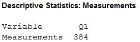
From the output the first quartile is 384.
g.
Compute the third quartile.
Answer to Problem 16SE
The third quartile is 1,018.
Explanation of Solution
Calculation:
Step by step procedure for finding the third quartile of the concentration is follows:
- Choose Stat > Basic Statistics > Display Descriptive Statistics.
- In Variables enter the columns Measurements.
- Choose option statistics, and select Third quartile.
- Click OK.
Output using Minitab software is,
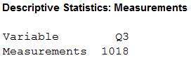
From the output the third quartile is 1,018.
h.
Compute the interquartile range.
Answer to Problem 16SE
The interquartile range is 634.
Explanation of Solution
Calculation:
Step by step procedure for finding the third quartile of the concentration is follows:
- Choose Stat > Basic Statistics > Display Descriptive Statistics.
- In Variables enter the columns Measurements.
- Choose option statistics, and select Interquartile range.
- Click OK.
Output using Minitab software is,
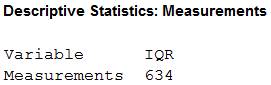
From the output the interquartile range is 634.
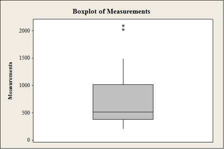
i.
Construct a boxplot for the concentrations.
Answer to Problem 16SE
The boxplot for the given data is,
Explanation of Solution
Calculation:
Step by step procedure to constructing boxplot using Minitab procedure is follows:
- Choose Graph > Boxplot or Stat > EDA > Boxplot.
- Under One Y, choose Simple. Click OK.
- In Graph variables, enter Measurements.
- Click OK.
j.
Identify the points in any outliers.
Answer to Problem 16SE
The points 2,030 and 2,099 are outliers.
Explanation of Solution
Calculation:
Outlier:
If the sample contain a few points that are much larger or smaller than the rest then the points are called outliers.
From the boxplot, it can be concluded that there are two outliers. They are 2,030 and 2,099.
k.
Identify it is skewed to the left, skewed to the right or approximately symmetric if histogram were constructed.
Answer to Problem 16SE
The histogram is skewed to the right.
Explanation of Solution
Calculation:
Left and Right skewed:
If the sample is left skewed then the median is closer to the third quartile than to the first quartile and if the sample is right skewed then the median is closer to the first quartile than to the third quartile.
From the boxplot, it is observed that the median is closer to the first quartile than to the third quartile. That is, the data is skewed to the right.
Therefore, the histogram is skewed to the right.
Want to see more full solutions like this?
Chapter 1 Solutions
EBK STATISTICS FOR ENGINEERS AND SCIENT


- You find out that the dietary scale you use each day is off by a factor of 2 ounces (over — at least that’s what you say!). The margin of error for your scale was plus or minus 0.5 ounces before you found this out. What’s the margin of error now?arrow_forwardSuppose that Sue and Bill each make a confidence interval out of the same data set, but Sue wants a confidence level of 80 percent compared to Bill’s 90 percent. How do their margins of error compare?arrow_forwardSuppose that you conduct a study twice, and the second time you use four times as many people as you did the first time. How does the change affect your margin of error? (Assume the other components remain constant.)arrow_forward
- Out of a sample of 200 babysitters, 70 percent are girls, and 30 percent are guys. What’s the margin of error for the percentage of female babysitters? Assume 95 percent confidence.What’s the margin of error for the percentage of male babysitters? Assume 95 percent confidence.arrow_forwardYou sample 100 fish in Pond A at the fish hatchery and find that they average 5.5 inches with a standard deviation of 1 inch. Your sample of 100 fish from Pond B has the same mean, but the standard deviation is 2 inches. How do the margins of error compare? (Assume the confidence levels are the same.)arrow_forwardA survey of 1,000 dental patients produces 450 people who floss their teeth adequately. What’s the margin of error for this result? Assume 90 percent confidence.arrow_forward
- The annual aggregate claim amount of an insurer follows a compound Poisson distribution with parameter 1,000. Individual claim amounts follow a Gamma distribution with shape parameter a = 750 and rate parameter λ = 0.25. 1. Generate 20,000 simulated aggregate claim values for the insurer, using a random number generator seed of 955.Display the first five simulated claim values in your answer script using the R function head(). 2. Plot the empirical density function of the simulated aggregate claim values from Question 1, setting the x-axis range from 2,600,000 to 3,300,000 and the y-axis range from 0 to 0.0000045. 3. Suggest a suitable distribution, including its parameters, that approximates the simulated aggregate claim values from Question 1. 4. Generate 20,000 values from your suggested distribution in Question 3 using a random number generator seed of 955. Use the R function head() to display the first five generated values in your answer script. 5. Plot the empirical density…arrow_forwardFind binomial probability if: x = 8, n = 10, p = 0.7 x= 3, n=5, p = 0.3 x = 4, n=7, p = 0.6 Quality Control: A factory produces light bulbs with a 2% defect rate. If a random sample of 20 bulbs is tested, what is the probability that exactly 2 bulbs are defective? (hint: p=2% or 0.02; x =2, n=20; use the same logic for the following problems) Marketing Campaign: A marketing company sends out 1,000 promotional emails. The probability of any email being opened is 0.15. What is the probability that exactly 150 emails will be opened? (hint: total emails or n=1000, x =150) Customer Satisfaction: A survey shows that 70% of customers are satisfied with a new product. Out of 10 randomly selected customers, what is the probability that at least 8 are satisfied? (hint: One of the keyword in this question is “at least 8”, it is not “exactly 8”, the correct formula for this should be = 1- (binom.dist(7, 10, 0.7, TRUE)). The part in the princess will give you the probability of seven and less than…arrow_forwardplease answer these questionsarrow_forward
- Selon une économiste d’une société financière, les dépenses moyennes pour « meubles et appareils de maison » ont été moins importantes pour les ménages de la région de Montréal, que celles de la région de Québec. Un échantillon aléatoire de 14 ménages pour la région de Montréal et de 16 ménages pour la région Québec est tiré et donne les données suivantes, en ce qui a trait aux dépenses pour ce secteur d’activité économique. On suppose que les données de chaque population sont distribuées selon une loi normale. Nous sommes intéressé à connaitre si les variances des populations sont égales.a) Faites le test d’hypothèse sur deux variances approprié au seuil de signification de 1 %. Inclure les informations suivantes : i. Hypothèse / Identification des populationsii. Valeur(s) critique(s) de Fiii. Règle de décisioniv. Valeur du rapport Fv. Décision et conclusion b) A partir des résultats obtenus en a), est-ce que l’hypothèse d’égalité des variances pour cette…arrow_forwardAccording to an economist from a financial company, the average expenditures on "furniture and household appliances" have been lower for households in the Montreal area than those in the Quebec region. A random sample of 14 households from the Montreal region and 16 households from the Quebec region was taken, providing the following data regarding expenditures in this economic sector. It is assumed that the data from each population are distributed normally. We are interested in knowing if the variances of the populations are equal. a) Perform the appropriate hypothesis test on two variances at a significance level of 1%. Include the following information: i. Hypothesis / Identification of populations ii. Critical F-value(s) iii. Decision rule iv. F-ratio value v. Decision and conclusion b) Based on the results obtained in a), is the hypothesis of equal variances for this socio-economic characteristic measured in these two populations upheld? c) Based on the results obtained in a),…arrow_forwardA major company in the Montreal area, offering a range of engineering services from project preparation to construction execution, and industrial project management, wants to ensure that the individuals who are responsible for project cost estimation and bid preparation demonstrate a certain uniformity in their estimates. The head of civil engineering and municipal services decided to structure an experimental plan to detect if there could be significant differences in project evaluation. Seven projects were selected, each of which had to be evaluated by each of the two estimators, with the order of the projects submitted being random. The obtained estimates are presented in the table below. a) Complete the table above by calculating: i. The differences (A-B) ii. The sum of the differences iii. The mean of the differences iv. The standard deviation of the differences b) What is the value of the t-statistic? c) What is the critical t-value for this test at a significance level of 1%?…arrow_forward
 MATLAB: An Introduction with ApplicationsStatisticsISBN:9781119256830Author:Amos GilatPublisher:John Wiley & Sons Inc
 Probability and Statistics for Engineering and th...StatisticsISBN:9781305251809Author:Jay L. DevorePublisher:Cengage Learning
 Statistics for The Behavioral Sciences (MindTap C...StatisticsISBN:9781305504912Author:Frederick J Gravetter, Larry B. WallnauPublisher:Cengage Learning
 Elementary Statistics: Picturing the World (7th E...StatisticsISBN:9780134683416Author:Ron Larson, Betsy FarberPublisher:PEARSON
 The Basic Practice of StatisticsStatisticsISBN:9781319042578Author:David S. Moore, William I. Notz, Michael A. FlignerPublisher:W. H. Freeman
 Introduction to the Practice of StatisticsStatisticsISBN:9781319013387Author:David S. Moore, George P. McCabe, Bruce A. CraigPublisher:W. H. Freeman