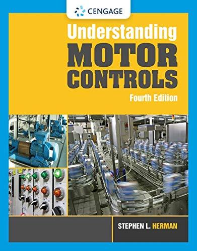
Algorithm 3 Discrete-time system matrix computation (assuming ZOH control) Input: tk, tk+1, Yk = [x, vec(In), 0+x] 1: traj ode45(@(t,Y) EoMwithDiscrete Matrix(t, Y, Uk), [tk, tk+1), Yk) 2: Yk+1deval (traj, tk+1) 3: k+1Yk+1(1: n₂) 4: A 5: Bk reshape(Yk+1(nx +1: n + n²), nx, nx) * Ak [reshape(Yk+1(n + n + 1 : n₂+n² + n₂Nu), Nx, Nu)] 6: Ck ← Ak * [Yk+1(Nx + n² + NxNu + 1 : nx + n² + nxnu + nx)] ▷ Integrate Y over [tk, tk+1) Obtain Y evaluated at tk+1 Algorithm 4 EoMwith Discrete Matrix Input: t, Y, uk, Output: Y 1: 2: Y(1x) reshape(Y(nx + 1 : nr + n²), nz, nx) f(x) 8x f(x,uk,t) vec(A) 3: A 4: Y← vec(-¹B) Bf, c+f(x, uk, t) - Ax - Buk Ju ▷ same as (t, tk) ▷same as A(t), B(t), c(t) vec(-¹c)]


I need help with a MATLAB code. I am trying to implement algorithm 3 and 4 as shown in the image. I am getting some size errors. Can you help me fix the code.
clc;
clear all;
% Define initial conditions and parameters
r0 = [1000, 0, 0]; % Initial position in meters
v0 = [0, 10, 0]; % Initial velocity in m/s
m0 = 1000; % Initial mass in kg
z0 = log(m0); % Initial mass logarithm
a0 = [0, 0, 1]; % Initial thrust direction in m/s^2 (thrust in z-direction)
sigma0 = 0.1; % Initial thrust magnitude divided by mass
% Initial state
x0 = [r0, v0, z0];
% Initial control input u0 = [a0, sigma0]
u0 = [a0, sigma0];
% Time span for integration
t0 = 0; % Initial time
tf = 10; % Final time
N = 100; % Number of time steps
dt = (tf - t0) / N; % Time step size
t_span = linspace(t0, tf, N); % Discretized time vector
% Solve the system of equations using ode45
[t, Y] = ode45(@(t, Y) EoMwithDiscreteMatrix(t, Y, u0, x0, t0, tf), t_span, x0);
% Compute the matrices A_k, B_k, and c_k using the system's equations of motion
[A_k, B_k, c_k] = computeDiscreteMatrices(t_span, x0, Y, u0);
% Display the values for A_k, B_k, and c_k
disp('A_k:');
disp(A_k);
disp('B_k:');
disp(B_k);
disp('c_k:');
disp(c_k);
% Objective function J (total thrust over time)
J = sum(sigma0 * dt); % Assuming constant sigma over the time steps
disp('Objective Function J:');
disp(J);
%% Function to compute the system matrices A, B, and c at each time step
function Y_dot = EoMwithDiscreteMatrix(t, Y, u, x, tk, tkp1)
% Ensure the correct size for the state vector
n = 7; % State vector dimension (r, v, z)
n2 = length(u); % Control vector dimension (a, sigma)
% Ensure that Y has the expected dimensions (n x 1)
if length(Y) ~= n
error('Y does not have the expected dimensions');
end
% Extract the state vector (position, velocity, mass)
r = Y(1:3); % Position vector (3x1)
v = Y(4:6); % Velocity vector (3x1)
z = Y(7); % Logarithm of mass (1x1)
% Compute A, B, and c based on the system dynamics
A = df_dx(Y(1:n), u); % df/dx at current state
B = df_du(Y(1:n), u); % df/du at current state
% Compute the nonlinearities (additional forces)
c = f(Y(1:n), u, t) - A*Y(1:n) - B*u';
% Compute the state transition matrix (Phi)
Phi = reshape(Y(1:n), n, n); % Reshape Y appropriately
% Compute Y_dot for integration
Y_dot = [f(Y(1:n), u, t); A*Y(1:n) + B*u']; % Dynamics update rule
end
%% Function to compute the system matrices at each time step
function [A_k, B_k, c_k] = computeDiscreteMatrices(t_span, x0, Y, u0)
% Algorithm 3 - Discrete-time system matrix computation
n = length(x0); % State dimension (e.g., 7 for r, v, z)
n2 = length(u0); % Control dimension (e.g., 2 for a, sigma)
% Ensure that Y has the correct size
if size(Y, 2) ~= n
error('Y does not have the expected dimensions for state variables');
end
% Compute x_k and other parameters for matrix calculation
x_k = Y(:,1:n);
A_k = reshape(Y(:,n+1:n+n2), n, n); % Reshape to get matrix A_k
B_k = reshape(Y(:,n+n2+1:n+n2+n2), n, n2); % Reshape to get matrix B_k
c_k = A_k * Y(:,n+n2+1:end); % Compute nonlinearities matrix c_k
end
%% Dummy functions (Replace with your specific system dynamics)
function A = df_dx(x, u)
% Compute df/dx (state-space matrix A)
A = eye(length(x)); % Replace with actual computation
end
function B = df_du(x, u)
% Compute df/du (control matrix B)
B = eye(length(u)); % Replace with actual computation
end
function c = f(x, u, t)
% Compute the nonlinearities (force, etc.)
c = zeros(length(x), 1); % Replace with actual computation
end
![Algorithm 3 Discrete-time system matrix computation (assuming ZOH control)
Input: tk, tk+1, Yk = [x, vec(In), 0+x]
1: traj ode45(@(t,Y) EoMwithDiscrete Matrix(t, Y, Uk), [tk, tk+1), Yk)
2: Yk+1deval (traj, tk+1)
3: k+1Yk+1(1: n₂)
4: A
5: Bk
reshape(Yk+1(nx +1: n + n²), nx, nx)
*
Ak [reshape(Yk+1(n + n + 1 : n₂+n² + n₂Nu), Nx, Nu)]
6: Ck ← Ak * [Yk+1(Nx + n² + NxNu + 1 : nx + n² + nxnu + nx)]
▷ Integrate Y over [tk, tk+1)
Obtain Y evaluated at tk+1](/v2/_next/image?url=https%3A%2F%2Fcontent.bartleby.com%2Fqna-images%2Fquestion%2Fad0d55fe-d83b-4711-86a1-cee8ecea510f%2Fb8e5c957-a7ad-46a3-867f-578a16dbbd35%2F1xnlpcg_processed.png&w=3840&q=75)
![Algorithm 4 EoMwith Discrete Matrix
Input: t, Y, uk, Output: Y
1:
2:
Y(1x)
reshape(Y(nx + 1 : nr + n²), nz, nx)
f(x)
8x
f(x,uk,t)
vec(A)
3: A
4: Y←
vec(-¹B)
Bf, c+f(x, uk, t) - Ax - Buk
Ju
▷ same as (t, tk)
▷same as A(t), B(t), c(t)
vec(-¹c)]](/v2/_next/image?url=https%3A%2F%2Fcontent.bartleby.com%2Fqna-images%2Fquestion%2Fad0d55fe-d83b-4711-86a1-cee8ecea510f%2Fb8e5c957-a7ad-46a3-867f-578a16dbbd35%2Fzeiqk3_processed.png&w=3840&q=75)

Step by step
Solved in 2 steps with 2 images