a.
To evaluate the marginal revenue and Average revenue functions from the table given in the question.
a.
Explanation of Solution
Average revenue is the revenue which is obtained by dividing total revenue by quantity.
Marginal revenue is the additional revenue which is obtained by selling an extra unit of the product.
Formula to find the Marginal revenue (MR) and Average revenue (AR)
| Output | Total Revenue (TR) | Marginal Revenue | Average Revenue |
| 0 | 0 | - | - |
| 1 | 34 |
|
|
| 2 | 66 |
|
|
| 3 | 96 | 30 | 32 |
| 4 | 124 | 28 | 31 |
| 5 | 150 | 26 | 30 |
| 6 | 174 | 24 | 29 |
| 7 | 196 | 22 | 28 |
| 8 | 216 | 20 | 27 |
| 9 | 234 | 18 | 26 |
| 10 | 250 | 16 | 25 |
| 11 | 264 | 14 | 24 |
| 12 | 276 | 12 | 23 |
| 13 | 286 | 10 | 22 |
| 14 | 294 | 8 | 21 |
| 15 | 300 | 6 | 20 |
| 16 | 304 | 4 | 19 |
| 17 | 306 | 2 | 18 |
| 18 | 306 | 0 | 17 |
| 19 | 304 | -2 | 16 |
| 20 | 300 | -4 | 15 |
Introduction: Average revenue is revenue produced per unit of product sold. It plays a part in deciding the income for a company. The average revenue is less than the average (total) expense per unit income. An organization typically aims to generate the amount of production that maximizes income.
b.
To evaluate the marginal cost and Average cost functions from the table given in the question.
b.
Explanation of Solution
Formula to find the MC and AC are:
| Output | Total Cost (TC) | Marginal Cost | Average Revenue |
| 0 | 20 | - | - |
| 1 | 26 |
|
|
| 2 | 34 |
|
|
| 3 | 44 | 10 | 14.7 |
| 4 | 56 | 12 | 14.0 |
| 5 | 70 | 14 | 14.0 |
| 6 | 86 | 16 | 14.3 |
| 7 | 104 | 18 | 14.9 |
| 8 | 124 | 20 | 15.5 |
| 9 | 146 | 22 | 16.2 |
| 10 | 170 | 24 | 17.0 |
| 11 | 196 | 26 | 17.8 |
| 12 | 224 | 28 | 18.7 |
| 13 | 254 | 30 | 19.5 |
| 14 | 286 | 32 | 20.4 |
| 15 | 320 | 34 | 21.3 |
| 16 | 356 | 36 | 22.3 |
| 17 | 394 | 38 | 23.2 |
| 18 | 434 | 40 | 24.1 |
| 19 | 476 | 42 | 25.1 |
| 20 | 520 | 44 | 26.0 |
Introduction: The average cost method assigns a cost to inventory items based on the overall cost of the produced or manufactured goods over a period divided by the total number of products purchased or made. Often known as weighted-average method, is the average cost method.
c.
To evaluate the point where MR = MC and the output level in the graph that maximizes profits.
c.
Explanation of Solution
In economics, profit maximization is the short-term or long-term mechanism by which a firm can decide the levels of price, input, and production that lead to the highest benefit.
The graph is shown below:
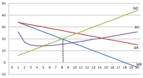
Marginal revenue equals to Marginal cost when Output (Q) = 8, where MC = MR =20
Introduction: Marginal revenue is the rise in revenue arising from the selling of one extra output unit. Although marginal revenue may remain constant for a certain level of production, the law of diminishing returns follows and inevitably slows down as the level of production increases.
d.
To evaluate the point where MR = MC and the output level in the graph that maximizes profits.s
d.
Explanation of Solution
The average cost method assigns a cost to inventory items based on the overall cost of the produced or manufactured goods over a period divided by the total number of products purchased or made. Often known as weighted-average method, is the average cost method.
In economics, profit maximization is the short-term or long-term mechanism by which a firm can decide the levels of price, input, and production that lead to the highest benefit.
Referring from the tables in part (a) and part (b) and the solution at Q = 8, the table is given below:
| Output | Marginal Cost | Marginal Revenue |
| 8 | 20 | 20 |
Introduction: Marginal revenue is the rise in revenue arising from the selling of one extra output unit. Although marginal revenue may remain constant for a certain level of production, the law of diminishing returns follows and inevitably slows down as the level of production increases. Perfectly competitive firms continue to generate production until marginal revenue is equal to marginal costs.
Want to see more full solutions like this?
Chapter B Solutions
Managerial Economics: Applications, Strategies and Tactics (MindTap Course List)

- refer to exhibit 8.12 and identify each curve in the grapharrow_forwardQ1. (Chap 1: Game Theory.) In the simultaneous games below player 1 is choosing between Top and Bottom, while player 2 is choosing between Left and Right. In each cell the first number is the payoff to player 1 and the second is the payoff to player 2. Part A: Player 1 Top Bottom Player 2 Left 25, 22 Right 27,23 26,21 28, 22 (A1) Does player 1 have a dominant strategy? (Yes/No) If your answer is yes, which one is it? (Top/Bottom) (A2) Does player 2 have a dominant strategy? (Yes/No.) If your answer is yes, which one is it? (Left/Right.) (A3) Can you solve this game by using the dominant strategy method? (Yes/No) If your answer is yes, what is the solution?arrow_forwardnot use ai pleasearrow_forward
- subject to X1 X2 Maximize dollars of interest earned = 0.07X1+0.11X2+0.19X3+0.15X4 ≤ 1,000,000 <2,500,000 X3 ≤ 1,500,000 X4 ≤ 1,800,000 X3 + XA ≥ 0.55 (X1+X2+X3+X4) X1 ≥ 0.15 (X1+X2+X3+X4) X1 + X2 X3 + XA < 5,000,000 X1, X2, X3, X4 ≥ 0arrow_forwardnot use aiarrow_forwardPlease help and Solve! (Note: this is a practice problem)arrow_forward
- Please help and thanks! (Note: This is a practice problem!)arrow_forwardUnit VI Assignment Instructions: This assignment has two parts. Answer the questions using the charts. Part 1: Firm 1 High Price Low Price High Price 8,8 0,10 Firm 2 Low Price 10,0 3,3 Question: For the above game, identify the Nash Equilibrium. Does Firm 1 have a dominant strategy? If so, what is it? Does Firm 2 have a dominant strategy? If so, what is it? Your response:arrow_forwardnot use ai please don't kdjdkdkfjnxncjcarrow_forward
- Ask one question at a time. Keep questions specific and include all details. Need more help? Subject matter experts with PhDs and Masters are standing by 24/7 to answer your question.**arrow_forward1b. (5 pts) Under the 1990 Farm Bill and given the initial situation of a target price and marketing loan, indicate where the market price (MP), quantity supplied (QS) and demanded (QD), government stocks (GS), and Deficiency Payments (DP) and Marketing Loan Gains (MLG), if any, would be on the graph below. If applicable, indicate the price floor (PF) on the graph. TP $ NLR So Do Q/yrarrow_forwardNow, let us assume that Brie has altruistic preferences. Her utility function is now given by: 1 UB (xA, YA, TB,YB) = (1/2) (2x+2y) + (2x+2y) What would her utility be at the endowment now? (Round off your answer to the nearest whole number.) 110arrow_forward
 Managerial Economics: Applications, Strategies an...EconomicsISBN:9781305506381Author:James R. McGuigan, R. Charles Moyer, Frederick H.deB. HarrisPublisher:Cengage Learning


 Managerial Economics: A Problem Solving ApproachEconomicsISBN:9781337106665Author:Luke M. Froeb, Brian T. McCann, Michael R. Ward, Mike ShorPublisher:Cengage Learning