
a
To plot:
Graphical representation of isoquant and quantity of K and L.
a
Explanation of Solution
Since q = 40,000 has been produced with
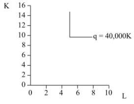
In the above diagram, x-axis measures labor while y-axis measures capital, q represents isoquant of Large Mowers as depicted above.
Introduction:
Isoquant curve is a graphical representation showing the same level of output production with different combinations of inputs.
b)
To plot:
Graphical function of isoquant for small mower.
b)
Explanation of Solution
This diagram shows the plotting of q = 40,000, K = 8 and L = 8
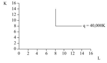
In the above diagram, x-axis measures labor while the y-axis measures capital. Q represents isoquant of Small Mowers as depicted above.
Introduction:
Expansion path is a combination of optimal output when input changes due to prices.
c)
To know:
Quantities of K and L for different lawn divisions.
c)
Explanation of Solution
Production functions are given below:
When lawn is cut by 1st method:
When lawn is cut by 2nd method:
Total capital requirement = 9
Total labor requirement = 6.5
Production functions are given below:
When lawn is cut by 1st method:
When lawn is cut by 2nd method:
Total capital requirement = 9.5
Total labor requirement = 5.75
The fraction of K and L means the amount of capital input used per unit of labor.
This table shows the resources uses in the Large Mowers and Small Mowers.
| 40,000 sq.ft. | LM | SM | ||
| LM/SM mix | L | K | L | K |
| 0/100$% | 0 | 0 | 8 | 8 |
| 25%/75% | 1.25 | 2.5 | 6 | 6 |
| 50%/50% | 2.5 | 5 | 4 | 4 |
| 75%/25% | 3.75 | 7.5 | 2 | 2 |
| 100%/0% | 5 | 10 | 0 | 0 |
Introduction:
Isoquant curve is a graphical representation showing the same level of output production with different combinations of inputs.
d)
To plot:
Graphical representation of isoquant.
d)
Explanation of Solution
Calculation of labor and capital when 40000 square foot of lawn is cut by 1st method with p fraction.
Calculation of labor and capital when (1-p) fraction of 40,000 square foot lawn is cut by 2nd method.
Calculation of labor requirement:
Calculation of total capital requirement:
Two equations are given as follows:
Solving first equation for p and putting the value of p in second as shown below:
The Table shows the different calculations of Labor (L) and capital (K) in Small Mowers as shown below:
| 40,000 sq.ft. | LM | |
| LM/SM mix | L | K |
| 0/100$% | 8 | 8 |
| 25%/75% | 7.25 | 8.5 |
| 50%/50% | 6.5 | 9 |
| 75%/25% | 5.75 | 9.5 |
| 100%/0% | 5 | 10 |
Following graph is plotted from the given table shows the isoquant for the combined production function as shown below:
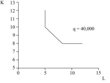
In the above diagram, x-axis measures labor while y-axis measures capital, q represents isoquant for the combined production function as depicted above.
Introduction:
Expansion path is a combination of optimal output when input changes due to prices.
Want to see more full solutions like this?
Chapter 9 Solutions
EBK MICROECONOMIC THEORY: BASIC PRINCIP

- Section III: Empirical Findings: Descriptive Statistics and inferential statistics………………..40% Descriptive statistics provide details about the Y variable, based on the sample for the 10-year period. Here, you use Excell or manually compute Mean or the average income per capita. Interpret the meaning of average income per capita. Draw the line chart showing the educational performance over the time-period of your study. Label the Vertical axis as Y performance and X axis as the explanatory variable (X1) . Do the same thing between Y and X2 Empirical/ Inferential Statistics: Here, use the sample information to perform the following: Draw the Scatter plot and impose the trend line: showing the Y variable and explanatory variables ( X1). Draw the scatter plot and impose the tend line: Showing Y and X2. Does your evidence (data) support your theory? Refer to the trend line: Is the relationship positive or negative as expected? Create graphs based on table below; Years Y ( per…arrow_forwardPlease help me with this Accounting questionarrow_forwardTitle: Does the educational performance depend on its literacy rate and government spending over the last 10 years? In the introduction, there are four things to include:a) Clearly state your research topic follows by country’s background in terms of (population density; male/female ratio; and identify the problem leading up to the study of it, such as government spending and adult literacy rate. How does the US perform compared to other countries.b) State the research question that you wish to resolve: Does the US economic performance depend on its government spending on education and the literacy rate over the last 10 years. Define performance (Y) as the average income per capita, an indicator of the country’s economy growing over time. For example, an increase in government spending leads to higher literacy rates and subsequently higher productivity in the economy. Also, mention that you will use a sample size of 10 years of secondary data from the existing literature,…arrow_forward
- Title: Does the educational performance depend on its literacy rate and government spending over the last 10 years? In the introduction, there are four things to include:a) Clearly state your research topic follows by country’s background in terms of (population density; male/female ratio; and identify the problem leading up to the study of it, such as government spending and adult literacy rate. How does the US perform compared to other countries.b) State the research question that you wish to resolve: Does the US economic performance depend on its government spending on education and the literacy rate over the last 10 years. Define performance (Y) as the average income per capita, an indicator of the country’s economy growing over time. For example, an increase in government spending leads to higher literacy rates and subsequently higher productivity in the economy. Also, mention that you will use a sample size of 10 years of secondary data from the existing literature,…arrow_forwardExplain how the introduction of egg replacers and plant-based egg products will impact the bakery industry. Provide a graphical representation.arrow_forwardExplain Professor Frederick's "cognitive reflection" test.arrow_forward
- 11:44 Fri Apr 4 Would+You+Take+the+Bird+in+the+Hand Would You Take the Bird in the Hand, or a 75% Chance at the Two in the Bush? BY VIRGINIA POSTREL WOULD you rather have $1,000 for sure or a 90 percent chance of $5,000? A guaranteed $1,000 or a 75 percent chance of $4,000? In economic theory, questions like these have no right or wrong answers. Even if a gamble is mathematically more valuable a 75 percent chance of $4,000 has an expected value of $3,000, for instance someone may still prefer a sure thing. People have different tastes for risk, just as they have different tastes for ice cream or paint colors. The same is true for waiting: Would you rather have $400 now or $100 every year for 10 years? How about $3,400 this month or $3,800 next month? Different people will answer differently. Economists generally accept those differences without further explanation, while decision researchers tend to focus on average behavior. In decision research, individual differences "are regarded…arrow_forwardDescribe the various measures used to assess poverty and economic inequality. Analyze the causes and consequences of poverty and inequality, and discuss potential policies and programs aimed at reducing them, assess the adequacy of current environmental regulations in addressing negative externalities. analyze the role of labor unions in labor markets. What is one benefit, and one challenge associated with labor unions.arrow_forwardEvaluate the effectiveness of supply and demand models in predicting labor market outcomes. Justify your assessment with specific examples from real-world labor markets.arrow_forward
- Explain the difference between Microeconomics and Macroeconomics? 2.) Explain what fiscal policy is and then explain what Monetary Policy is? 3.) Why is opportunity cost and give one example from your own of opportunity cost. 4.) What are models and what model did we already discuss in class? 5.) What is meant by scarcity of resources?arrow_forward2. What is the payoff from a long futures position where you are obligated to buy at the contract price? What is the payoff from a short futures position where you are obligated to sell at the contract price?? Draw the payoff diagram for each position. Payoff from Futures Contract F=$50.85 S1 Long $100 $95 $90 $85 $80 $75 $70 $65 $60 $55 $50.85 $50 $45 $40 $35 $30 $25 Shortarrow_forward3. Consider a call on the same underlier (Cisco). The strike is $50.85, which is the forward price. The owner of the call has the choice or option to buy at the strike. They get to see the market price S1 before they decide. We assume they are rational. What is the payoff from owning (also known as being long) the call? What is the payoff from selling (also known as being short) the call? Payoff from Call with Strike of k=$50.85 S1 Long $100 $95 $90 $85 $80 $75 $70 $65 $60 $55 $50.85 $50 $45 $40 $35 $30 $25 Shortarrow_forward

 Principles of Economics 2eEconomicsISBN:9781947172364Author:Steven A. Greenlaw; David ShapiroPublisher:OpenStax
 Microeconomics: Principles & PolicyEconomicsISBN:9781337794992Author:William J. Baumol, Alan S. Blinder, John L. SolowPublisher:Cengage Learning
 Exploring EconomicsEconomicsISBN:9781544336329Author:Robert L. SextonPublisher:SAGE Publications, Inc
