
INTRODUCTORY STAT. W/MYLAB MATH>CUSTOM<
3rd Edition
ISBN: 9780135231548
Author: Gould
Publisher: PEARSON C
expand_more
expand_more
format_list_bulleted
Concept explainers
Videos
Textbook Question
Chapter 9, Problem 41SE
Cholesterol In the U.S. Department of Health has suggested that a healthy total cholesterol measurement should be 200 mg/dL or less. Records from 50 randomly and independently selected people from the NHANES study showed the results in the Minitab output given:
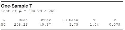
Test the hypothesis that the
Expert Solution & Answer
Want to see the full answer?
Check out a sample textbook solution
Students have asked these similar questions
Hi, I need to make sure I have drafted a thorough analysis, so please answer the following questions. Based on the data in the attached image, develop a regression model to forecast the average sales of football magazines for each of the seven home games in the upcoming season (Year 10). That is, you should construct a single regression model and use it to estimate the average demand for the seven home games in Year 10. In addition to the variables provided, you may create new variables based on these variables or based on observations of your analysis. Be sure to provide a thorough analysis of your final model (residual diagnostics) and provide assessments of its accuracy. What insights are available based on your regression model?
I want to make sure that I included all possible variables and observations. There is a considerable amount of data in the images below, but not all of it may be useful for your purposes. Are there variables contained in the file that you would exclude from a forecast model to determine football magazine sales in Year 10? If so, why? Are there particular observations of football magazine sales from previous years that you would exclude from your forecasting model? If so, why?
Stat questions
Chapter 9 Solutions
INTRODUCTORY STAT. W/MYLAB MATH>CUSTOM<
Ch. 9 - Ages A study of all the students at a small...Ch. 9 - Units A survey of 100 random full-time students at...Ch. 9 - Exam Scores The distribution of the scores on a...Ch. 9 - Exam Scores The distribution of the scores on a...Ch. 9 - Showers According to home-water-works.org, the...Ch. 9 - Smartphones According to a 2017 report by ComScore...Ch. 9 - Retirement Income Several times during the year,...Ch. 9 - Time Employed A human resources manager for a...Ch. 9 - Driving (Example 1) Drivers in Wyoming drive more...Ch. 9 - Driving Drivers in Alaska drive fewer miles yearly...
Ch. 9 - Babies Weights (Example 2) Some sources report...Ch. 9 - Babies’ Weights, Again Some sources report that...Ch. 9 - (Example 3) Income in Maryland According to a 2018...Ch. 9 - Income in Kansas According to a 2018 Money...Ch. 9 - CLT Shapes (Example 4) One of the histograms is a...Ch. 9 - Used Van Costs One histogram shows the...Ch. 9 - (Example 5) Age of Used Vans The mean age of all...Ch. 9 - Student Ages The mean age of all 2550 students at...Ch. 9 - Prob. 19SECh. 9 - Prob. 20SECh. 9 - Prob. 21SECh. 9 - Prob. 22SECh. 9 - Private University Tuition (Example 7) A random...Ch. 9 - Random Numbers If you take samples of 40 lines...Ch. 9 - t* (Example 8) A researcher collects one sample of...Ch. 9 - t* A researcher collects a sample of 25...Ch. 9 - Heights of 12th Graders (Example 9) A random...Ch. 9 - Drinks A fast-food chain sells drinks that it...Ch. 9 - Men’s Pulse Rates (Example 10) A random sample of...Ch. 9 - Travel Time to School A random sample of 50...Ch. 9 - RBIs (Example 11) A random sample of 25 baseball...Ch. 9 - RBIs Again In exercise 9.31, two intervals were...Ch. 9 - Confidence Interval Changes State whether each of...Ch. 9 - Confidence Interval Changes State whether each of...Ch. 9 - Potatoes The weights of four randomly and...Ch. 9 - Tomatoes The weights of four randomly and...Ch. 9 - Human Body Temperatures (Example 12) A random...Ch. 9 - Reaction Distance Data on the disk and website...Ch. 9 - Potatoes Use the data from exercise 9.35. a. If...Ch. 9 - Tomatoes Use the data from exercise 9.36. a. Using...Ch. 9 - Cholesterol In the U.S. Department of Health has...Ch. 9 - BMI A body mass index (BMI) of more than 25 is...Ch. 9 - Male Height In the United States, the population...Ch. 9 - Female Height In the United States, the population...Ch. 9 - Deflated Footballs? Patriots In the 2015 AFC...Ch. 9 - Deflated Footballs? Colts In the 2015 AFC...Ch. 9 - Movie Ticket Prices According to Deadline.com, the...Ch. 9 - Broadway Ticket Prices According to Statista.com,...Ch. 9 - Atkins Diet Difference Ten people went on an...Ch. 9 - Pulse Difference The following numbers are the...Ch. 9 - Student Ages Suppose that 200 statistics students...Ch. 9 - Presidents’ Ages at Inauguration A 95 confidence...Ch. 9 - Independent or Paired (Example 13) State whether...Ch. 9 - Independent or Paired State whether each situation...Ch. 9 - Televisions: CI (Example 14) Minitab output is...Ch. 9 - Pulse and Gender: CI Using data from NHANES, we...Ch. 9 - Televisions (Example 15) The table shows the...Ch. 9 - Pulse Rates Using data from NHANES, we looked at...Ch. 9 - Triglycerides Triglycerides are a form of fat...Ch. 9 - Systolic Blood Pressures When you have your blood...Ch. 9 - Triglycerides, Again Report and interpret the 95...Ch. 9 - Blood Pressures, Again Report and interpret the 95...Ch. 9 - Baseball Salaries A random sample of 40...Ch. 9 - College Athletes’ Weights A random sample of male...Ch. 9 - Baseball Salaries In exercise 9.63 you could not...Ch. 9 - College Athletes’ Weights In exercise 9.64, you...Ch. 9 - Textbook Prices, UCSB vs. CSUN (Example 16) The...Ch. 9 - Textbook Prices. OC vs. CSUN The prices of a...Ch. 9 - Females’ Pulse Rates before and after a Fright...Ch. 9 - Males’ Pulse Rates before and after a Fright...Ch. 9 - Organic Food A student compared organic food...Ch. 9 - Body Temperature The body temperatures of 65 men...Ch. 9 - Ales vs. IPAs Data were collected on calorie...Ch. 9 - Surfers Surfers and statistics students Rex...Ch. 9 - Self-Reported Heights of Men (Example 18) A random...Ch. 9 - Eating Out Jacqueline Loya, a statistics student,...Ch. 9 - Prob. 77SECh. 9 - Self-Driving Cars A survey of asked respondents...Ch. 9 - Women’s Heights Assume women’s heights are...Ch. 9 - Showers According to home-water-works.org, the...Ch. 9 - Choose a test for each situation: one-sample...Ch. 9 - Choose a t-test for each situation: one-sample...Ch. 9 - Cones: 3 Tests A McDonald’s fact sheet says its...Ch. 9 - Prob. 84CRECh. 9 - Brain Size Brain size for 20 random women and 20...Ch. 9 - Reducing Pollution A random sample of 12th-grade...Ch. 9 - Heart Rate before and after Coffee Elena Lucin, a...Ch. 9 - Exam Grades The final exam grades for a sample of...Ch. 9 - Hours of Television Viewing The number of hours...Ch. 9 - Reaction Distances Reaction distances in...Ch. 9 - Ales vs. Lagers Data were collected on calorie...Ch. 9 - Weights of Hockey and Baseball Players Data were...Ch. 9 - Grocery Delivery The table shows the prices for...Ch. 9 - Parents The following table shows the heights (in...Ch. 9 - Why Is n1 in the Sample Standard Deviation? Why do...Ch. 9 - Prob. 96CRECh. 9 - Construct two sets of body temperatures (in...Ch. 9 - Construct heights for 3 or more sets of twins (6...
Additional Math Textbook Solutions
Find more solutions based on key concepts
CHECK POINT I Consider the six jokes about books by Groucho Marx. Bob Blitzer. Steven Wright, HennyYoungman. Je...
Thinking Mathematically (6th Edition)
Provide an example of a qualitative variable and an example of a quantitative variable.
Elementary Statistics ( 3rd International Edition ) Isbn:9781260092561
Complete each statement with the correct term from the column on the right. Some of the choices may not be used...
Intermediate Algebra (13th Edition)
True or False The quotient of two polynomial expressions is a rational expression, (p. A35)
Precalculus
1. How is a sample related to a population?
Elementary Statistics: Picturing the World (7th Edition)
Is there a relationship between wine consumption and deaths from heart disease? The table gives data from 19 de...
College Algebra Essentials (5th Edition)
Knowledge Booster


Learn more about
Need a deep-dive on the concept behind this application? Look no further. Learn more about this topic, statistics and related others by exploring similar questions and additional content below.Similar questions
- 1) and let Xt is stochastic process with WSS and Rxlt t+t) 1) E (X5) = \ 1 2 Show that E (X5 = X 3 = 2 (= = =) Since X is WSSEL 2 3) find E(X5+ X3)² 4) sind E(X5+X2) J=1 ***arrow_forwardProve that 1) | RxX (T) | << = (R₁ " + R$) 2) find Laplalse trans. of Normal dis: 3) Prove thy t /Rx (z) | < | Rx (0)\ 4) show that evary algebra is algebra or not.arrow_forwardFor each of the time series, construct a line chart of the data and identify the characteristics of the time series (that is, random, stationary, trend, seasonal, or cyclical). Month Number (Thousands)Dec 1991 65.60Jan 1992 71.60Feb 1992 78.80Mar 1992 111.60Apr 1992 107.60May 1992 115.20Jun 1992 117.80Jul 1992 106.20Aug 1992 109.90Sep 1992 106.00Oct 1992 111.80Nov 1992 84.50Dec 1992 78.60Jan 1993 70.50Feb 1993 74.60Mar 1993 95.50Apr 1993 117.80May 1993 120.90Jun 1993 128.50Jul 1993 115.30Aug 1993 121.80Sep 1993 118.50Oct 1993 123.30Nov 1993 102.30Dec 1993 98.70Jan 1994 76.20Feb 1994 83.50Mar 1994 134.30Apr 1994 137.60May 1994 148.80Jun 1994 136.40Jul 1994 127.80Aug 1994 139.80Sep 1994 130.10Oct 1994 130.60Nov 1994 113.40Dec 1994 98.50Jan 1995 84.50Feb 1995 81.60Mar 1995 103.80Apr 1995 116.90May 1995 130.50Jun 1995 123.40Jul 1995 129.10Aug 1995…arrow_forward
- For each of the time series, construct a line chart of the data and identify the characteristics of the time series (that is, random, stationary, trend, seasonal, or cyclical). Year Month Units1 Nov 42,1611 Dec 44,1862 Jan 42,2272 Feb 45,4222 Mar 54,0752 Apr 50,9262 May 53,5722 Jun 54,9202 Jul 54,4492 Aug 56,0792 Sep 52,1772 Oct 50,0872 Nov 48,5132 Dec 49,2783 Jan 48,1343 Feb 54,8873 Mar 61,0643 Apr 53,3503 May 59,4673 Jun 59,3703 Jul 55,0883 Aug 59,3493 Sep 54,4723 Oct 53,164arrow_forwardHigh Cholesterol: A group of eight individuals with high cholesterol levels were given a new drug that was designed to lower cholesterol levels. Cholesterol levels, in milligrams per deciliter, were measured before and after treatment for each individual, with the following results: Individual Before 1 2 3 4 5 6 7 8 237 282 278 297 243 228 298 269 After 200 208 178 212 174 201 189 185 Part: 0/2 Part 1 of 2 (a) Construct a 99.9% confidence interval for the mean reduction in cholesterol level. Let a represent the cholesterol level before treatment minus the cholesterol level after. Use tables to find the critical value and round the answers to at least one decimal place.arrow_forwardI worked out the answers for most of this, and provided the answers in the tables that follow. But for the total cost table, I need help working out the values for 10%, 11%, and 12%. A pharmaceutical company produces the drug NasaMist from four chemicals. Today, the company must produce 1000 pounds of the drug. The three active ingredients in NasaMist are A, B, and C. By weight, at least 8% of NasaMist must consist of A, at least 4% of B, and at least 2% of C. The cost per pound of each chemical and the amount of each active ingredient in one pound of each chemical are given in the data at the bottom. It is necessary that at least 100 pounds of chemical 2 and at least 450 pounds of chemical 3 be used. a. Determine the cheapest way of producing today’s batch of NasaMist. If needed, round your answers to one decimal digit. Production plan Weight (lbs) Chemical 1 257.1 Chemical 2 100 Chemical 3 450 Chemical 4 192.9 b. Use SolverTable to see how much the percentage of…arrow_forward
- At the beginning of year 1, you have $10,000. Investments A and B are available; their cash flows per dollars invested are shown in the table below. Assume that any money not invested in A or B earns interest at an annual rate of 2%. a. What is the maximized amount of cash on hand at the beginning of year 4.$ ___________ A B Time 0 -$1.00 $0.00 Time 1 $0.20 -$1.00 Time 2 $1.50 $0.00 Time 3 $0.00 $1.90arrow_forwardFor each of the time series, construct a line chart of the data and identify the characteristics of the time series (that is, random, stationary, trend, seasonal, or cyclical). Year Month Rate (%)2009 Mar 8.72009 Apr 9.02009 May 9.42009 Jun 9.52009 Jul 9.52009 Aug 9.62009 Sep 9.82009 Oct 10.02009 Nov 9.92009 Dec 9.92010 Jan 9.82010 Feb 9.82010 Mar 9.92010 Apr 9.92010 May 9.62010 Jun 9.42010 Jul 9.52010 Aug 9.52010 Sep 9.52010 Oct 9.52010 Nov 9.82010 Dec 9.32011 Jan 9.12011 Feb 9.02011 Mar 8.92011 Apr 9.02011 May 9.02011 Jun 9.12011 Jul 9.02011 Aug 9.02011 Sep 9.02011 Oct 8.92011 Nov 8.62011 Dec 8.52012 Jan 8.32012 Feb 8.32012 Mar 8.22012 Apr 8.12012 May 8.22012 Jun 8.22012 Jul 8.22012 Aug 8.12012 Sep 7.82012 Oct…arrow_forwardFor each of the time series, construct a line chart of the data and identify the characteristics of the time series (that is, random, stationary, trend, seasonal, or cyclical). Date IBM9/7/2010 $125.959/8/2010 $126.089/9/2010 $126.369/10/2010 $127.999/13/2010 $129.619/14/2010 $128.859/15/2010 $129.439/16/2010 $129.679/17/2010 $130.199/20/2010 $131.79 a. Construct a line chart of the closing stock prices data. Choose the correct chart below.arrow_forward
- For each of the time series, construct a line chart of the data and identify the characteristics of the time series (that is, random, stationary, trend, seasonal, or cyclical) Date IBM9/7/2010 $125.959/8/2010 $126.089/9/2010 $126.369/10/2010 $127.999/13/2010 $129.619/14/2010 $128.859/15/2010 $129.439/16/2010 $129.679/17/2010 $130.199/20/2010 $131.79arrow_forward1. A consumer group claims that the mean annual consumption of cheddar cheese by a person in the United States is at most 10.3 pounds. A random sample of 100 people in the United States has a mean annual cheddar cheese consumption of 9.9 pounds. Assume the population standard deviation is 2.1 pounds. At a = 0.05, can you reject the claim? (Adapted from U.S. Department of Agriculture) State the hypotheses: Calculate the test statistic: Calculate the P-value: Conclusion (reject or fail to reject Ho): 2. The CEO of a manufacturing facility claims that the mean workday of the company's assembly line employees is less than 8.5 hours. A random sample of 25 of the company's assembly line employees has a mean workday of 8.2 hours. Assume the population standard deviation is 0.5 hour and the population is normally distributed. At a = 0.01, test the CEO's claim. State the hypotheses: Calculate the test statistic: Calculate the P-value: Conclusion (reject or fail to reject Ho): Statisticsarrow_forward21. find the mean. and variance of the following: Ⓒ x(t) = Ut +V, and V indepriv. s.t U.VN NL0, 63). X(t) = t² + Ut +V, U and V incepires have N (0,8) Ut ①xt = e UNN (0162) ~ X+ = UCOSTE, UNNL0, 62) SU, Oct ⑤Xt= 7 where U. Vindp.rus +> ½ have NL, 62). ⑥Xn = ΣY, 41, 42, 43, ... Yn vandom sample K=1 Text with mean zen and variance 6arrow_forward
arrow_back_ios
SEE MORE QUESTIONS
arrow_forward_ios
Recommended textbooks for you
 Glencoe Algebra 1, Student Edition, 9780079039897...AlgebraISBN:9780079039897Author:CarterPublisher:McGraw Hill
Glencoe Algebra 1, Student Edition, 9780079039897...
Algebra
ISBN:9780079039897
Author:Carter
Publisher:McGraw Hill
Probability & Statistics (28 of 62) Basic Definitions and Symbols Summarized; Author: Michel van Biezen;https://www.youtube.com/watch?v=21V9WBJLAL8;License: Standard YouTube License, CC-BY
Introduction to Probability, Basic Overview - Sample Space, & Tree Diagrams; Author: The Organic Chemistry Tutor;https://www.youtube.com/watch?v=SkidyDQuupA;License: Standard YouTube License, CC-BY