
Videos
Using Table G, find the critical value(s) for each. Show the critical and noncritical regions, and state the appropriate null and alternative hypotheses. Use σ2 = 225.
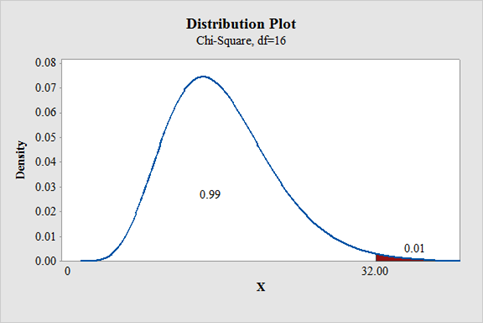
a. α = 0.01, n = 17, right-tailed
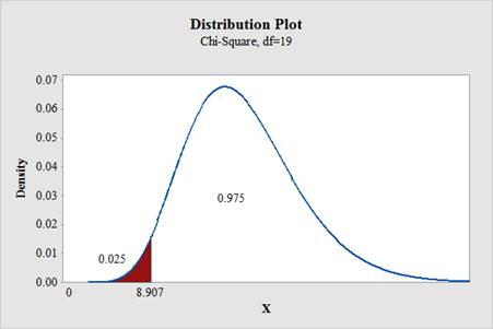
b. α = 0.025, n = 20, left-tailed
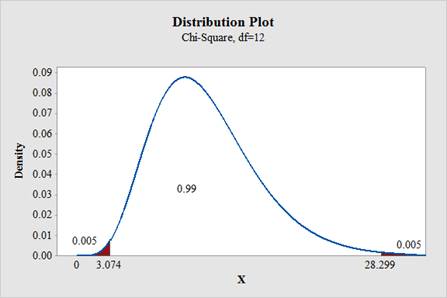
c. α = 0.01, n = 13, two-tailed
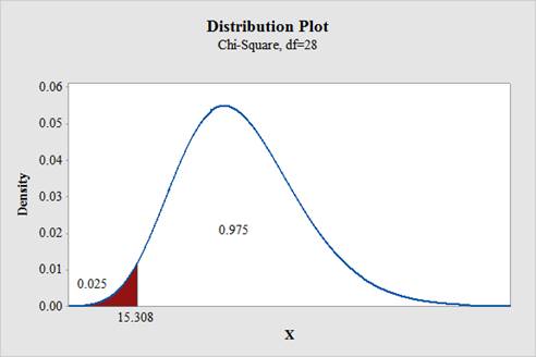
d. α = 0.025, n = 29, left-tailed
a.
To find: The critical value for right tailed test.
Answer to Problem 2E
The critical value for right tailed test is 32.000.
Null hypothesis:
Alternative hypothesis:
Explanation of Solution
The level of significance is
Answer:
Degrees of freedom:
From “Table G: The chi square distribution”, the critical values for the
Software Procedure:
Degrees of freedom:
From “Table G: The chi square distribution”, the critical values for the
Software Procedure:
Step-by-step procedure to obtain the critical region using the MINITAB software:
- Choose Graph > Probability Distribution Plot > choose View Probability> OK.
- From Distribution, choose Chi-square.
- In Degrees of freedom, enter 16.
- Click the Shaded Area tab.
- Choose Probability value and Right Tail for the region of the curve to shade.
- Enter the Probability value as 0.01.
- Click OK.
Output using the MINITAB software is given below:
State the null and alternative hypotheses:
Null hypothesis:
Alternative hypothesis:
b.
To find: The critical value for left tailed test.
Answer to Problem 2E
The critical value for left tailed test is 8.907.
Null hypothesis:
Alternative hypothesis:
Explanation of Solution
The level of significance is
Solution:
Degrees of freedom:
If the test is left tail, the level of significance is subtracted from 1. That is,
From “Table G: The chi square distribution”, the critical values for the
Software Procedure:
Step-by-step procedure to obtain the critical region using the MINITAB software:
- Choose Graph > Probability Distribution Plot > choose View Probability> OK.
- From Distribution, choose Chi-square.
- In Degrees of freedom, enter 19.
- Click the Shaded Area tab.
- Choose Probability value and Left Tail for the region of the curve to shade.
- Enter the Probability value as 0.025.
- Click OK.
Output using the MINITAB software is given below:
State the null and alternative hypotheses:
Null hypothesis:
Alternative hypothesis:
c.
To find: The critical values for two tailed test.
Answer to Problem 2E
The critical values for two tailed test is 3.074 and 28.299, respectively.
Null hypothesis:
Alternative hypothesis:
Explanation of Solution
Given info:
The level of significance is
Solution:
Degrees of freedom:
The area to the right of larger value is,
From “Table G: The chi square distribution”, the critical values for the
Software Procedure:
Step-by-step procedure to obtain the critical region using the MINITAB software:
- Choose Graph > Probability Distribution Plot > choose View Probability> OK.
- From Distribution, choose Chi-square.
- In Degrees of freedom, enter 12.
- Click the Shaded Area tab.
- Choose Probability value and Both Tail for the region of the curve to shade.
- Enter the Probability value as 0.01.
- Click OK.
Output using the MINITAB software is given below:
State the null and alternative hypotheses:
Null hypothesis:
Alternative hypothesis:
d.
To find: The critical value for left tailed test.
Answer to Problem 2E
The critical value for left tailed test is 15.308.
Null hypothesis:
Alternative hypothesis:
Explanation of Solution
Given info:
The level of significance is
Solution:
Degrees of freedom:
If the test is left tail, the level of significance is subtracted from 1. That is,
From “Table G: The chi square distribution”, the critical values for the
Software Procedure:
Step-by-step procedure to obtain the critical region using the MINITAB software:
- Choose Graph > Probability Distribution Plot > choose View Probability> OK.
- From Distribution, choose Chi-square.
- In Degrees of freedom, enter 28.
- Click the Shaded Area tab.
- Choose Probability value and Left Tail for the region of the curve to shade.
- Enter the Probability value as 0.025.
- Click OK.
Output using the MINITAB software is given below:
State the null and alternative hypotheses:
Null hypothesis:
Alternative hypothesis:
Want to see more full solutions like this?
Chapter 8 Solutions
Elementary Statistics: A Step By Step Approach


- A company found that the daily sales revenue of its flagship product follows a normal distribution with a mean of $4500 and a standard deviation of $450. The company defines a "high-sales day" that is, any day with sales exceeding $4800. please provide a step by step on how to get the answers in excel Q: What percentage of days can the company expect to have "high-sales days" or sales greater than $4800? Q: What is the sales revenue threshold for the bottom 10% of days? (please note that 10% refers to the probability/area under bell curve towards the lower tail of bell curve) Provide answers in the yellow cellsarrow_forwardFind the critical value for a left-tailed test using the F distribution with a 0.025, degrees of freedom in the numerator=12, and degrees of freedom in the denominator = 50. A portion of the table of critical values of the F-distribution is provided. Click the icon to view the partial table of critical values of the F-distribution. What is the critical value? (Round to two decimal places as needed.)arrow_forwardA retail store manager claims that the average daily sales of the store are $1,500. You aim to test whether the actual average daily sales differ significantly from this claimed value. You can provide your answer by inserting a text box and the answer must include: Null hypothesis, Alternative hypothesis, Show answer (output table/summary table), and Conclusion based on the P value. Showing the calculation is a must. If calculation is missing,so please provide a step by step on the answers Numerical answers in the yellow cellsarrow_forward
 Algebra & Trigonometry with Analytic GeometryAlgebraISBN:9781133382119Author:SwokowskiPublisher:Cengage