Operations Management: Processes and Supply Chains (12th Edition) (What's New in Operations Management)
12th Edition
ISBN: 9780134741062
Author: Lee J. Krajewski, Manoj K. Malhotra, Larry P. Ritzman
Publisher: PEARSON
expand_more
expand_more
format_list_bulleted
Concept explainers
Textbook Question
Chapter 8, Problem 7P
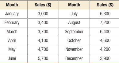
Sales for the past 12 months at Computer Success are given here. 
- Use a 3-month moving average to
forecast the sales for the months May through December. - Use a 4-month moving average to forecast the sales for the months May through December.
- Compare the performance of the two methods by using the mean absolute deviation as the performance criterion. Which method would you recommend?
- Compare the performance of the two methods by using the mean absolute percent error as the performance criterion. Which method would you recommend?
- Compare the performance of the two method by using the mean squared error as the performance criterion. Which method would you recommend?
Expert Solution & Answer
Want to see the full answer?
Check out a sample textbook solution
Students have asked these similar questions
Sales of tablet computers at Marika Gonzalez's electronics store in Washington, D.C., over the past 10 weeks are shown in the table below:
Week
1
2
3
4
5
6
7
8
9
10
Demand 21 21
27
38 25
30 35
24 25
30
a) The forecast for weeks 2 through 10 using exponential smoothing with a = 0.50 and a week 1 initial forecast of 21.0 are (round your responses to two decimal places):
Week
1
2
3
4
5
6
7
8
9
10
Demand 21
21
27
38 25
30
35
24 25 30
Forecast 21.0 21
21
24 31
28
29
32 28 26.50
b) For the forecast developed using exponential smoothing (a = 0.50 and initial forecast 21.0), the MAD = |||||sales (round your response to two decimal places).
Sales of tablet computers at Marika Gonzalez's electronics store in Washington, D.C., over the past 10 weeks are shown in the table below:
Week
Demand
1
2
3
4
5
6
7
8
9
10
21
21
27
38
25
30
35 24 25
30
a) The forecast for weeks 2 through 10 using exponential smoothing with a = 0.50 and a week 1 initial forecast of 21.0 are (round your responses to two decimal places):
Week
1
2
3
4
5
Demand 21 21
27 38
Forecast 21.0
☐ G
☐
☐
6
7
25 30 35
∞ ☐
8
9
10
24
25
30
Each machine costs $3 Million. Building the room with all its attendant safety protection and other ancillary costs increases the spending by an additional $2.0 million dollars per MRI suite. Each machine can perform 2000 scans per year.
Each reading of an MRI scan by a radiologist, along with other per-scan-related costs, is $500 per scan.
The machine will last five years.
Don’t worry about discount rates for this problem
Graph the total costs over 5 years as a function of sales for 0-3000 patients annually. Hint: you may need to add a second MRI at some point.
Suppose that you want to make a profit of $500 per scan at a target volume of 1000 patients per year, and you purchase only one machine. Superimpose the total revenue curve on top of the total cost curve in (1).
Chapter 8 Solutions
Operations Management: Processes and Supply Chains (12th Edition) (What's New in Operations Management)
Ch. 8 - Figure 8.9 shows summer air visibility...Ch. 8 - Kay and Michael Passe publish What‘s...Ch. 8 - Demand for oil changes at Garcia’s Garage has...Ch. 8 - Prob. 2PCh. 8 - Ohio Swiss Milk Products manufactures and...Ch. 8 - A manufacturing firm has developed a skills test,...Ch. 8 - The materials handling manager of a manufacturing...Ch. 8 - Marianne Kramer, the owner of Handy Man Rentals,...Ch. 8 - Sales for the past 12 months at Computer Success...Ch. 8 - Bradley’s Copiers sells and repairs photocopy...
Ch. 8 - Consider the sales data for Computer Success given...Ch. 8 - A convenience store recently started to carry a...Ch. 8 - Community Federal Bank in Dothan, Alabama,...Ch. 8 - The number of heart surgeries performed at...Ch. 8 - The following data are for calculator sales in...Ch. 8 - Prob. 14PCh. 8 - Forrest and Dan make boxes of chocolates for which...Ch. 8 - The manager of Alaina’s Garden Center must make...Ch. 8 - The manager of a utility company in the Texas...Ch. 8 - Franklin Tooling, Inc., manufactures specialty...Ch. 8 - Create an Excel spreadsheet on your own that can...Ch. 8 - Prob. 20PCh. 8 - Using the data in Problem 20 and the Time-Series...Ch. 8 - Prob. 22PCh. 8 - Cannister, Inc., specializes in the manufacture of...Ch. 8 - The Midwest Computer Company serves a large number...Ch. 8 - A certain food item at P=0.20 (with a combination...Ch. 8 - Prob. 26PCh. 8 - Prob. 27PCh. 8 - A manufacturing firm seeks to develop a better...Ch. 8 - How much does the forecasting process at Deckers...Ch. 8 - Prob. 2VCCh. 8 - What factors make forecasting at Deckers...Ch. 8 - Prob. 4VCCh. 8 - Prob. 5VCCh. 8 - Comment on the forecasting system being used by...Ch. 8 - Develop your own forecast for bow rakes for each...
Additional Business Textbook Solutions
Find more solutions based on key concepts
The flowchart for the process at the local car wash. Introduction: Flowchart: A flowchart is a visualrepresenta...
Principles of Operations Management: Sustainability and Supply Chain Management (10th Edition)
Real options and its types. Introduction: The net present value is the variation between present cash inflows v...
Gitman: Principl Manageri Finance_15 (15th Edition) (What's New in Finance)
Assume you are a CFO of a company that is attempting to race additional capital to finance an expansion of its ...
Financial Accounting, Student Value Edition (5th Edition)
A typical discounted price of a AAA battery is 0.75. It is designed to provide 1.5 volts and 1.0 amps for about...
Engineering Economy (17th Edition)
1-1. Define marketing and outline the steps in the marketing process. (AASCB: Communication)
Marketing: An Introduction (13th Edition)
How is activity-based costing useful for pricing decisions?
Horngren's Cost Accounting: A Managerial Emphasis (16th Edition)
Knowledge Booster
Learn more about
Need a deep-dive on the concept behind this application? Look no further. Learn more about this topic, operations-management and related others by exploring similar questions and additional content below.Similar questions
- I need the answer to requirement C.arrow_forwardImagine you are Susan Kim and are faced with a difficult choice to either follow the orders she was given, or refusing to do so. Using each lens determine what the ethical response would be. Suppot your answer with materials from readings and lectures. For example, using Universalism what would the ethical response be? Do the same for all four lenses.arrow_forwardAnswer all these questions, selecting any company of your choice. Choose a specific type of food company. Select a specific product. Develop all the inputs that are part of the process. Develop the transformation process in a graphic (diagram, etc.). Develop all the outputs or finished products that are part of the process. Describe all the processes involved in one line of production in any manufacturing facility. Also describing how good management is the center of any part of a production company.arrow_forward
- Using exponential smoothing with α =0.2, forecast the demand for The initial forecast for January is 2000 tons. Calculate the capacity utilization for June, July and Discuss the implications of underutilized or over utilized capacity for Green Harvestarrow_forwardIn organizational development when results are improving but relationships are declining, what leadership style is appropriate? directing delegating supporting coachingarrow_forwardWhat is the first thing a leader should do when moving through a cultural change? conduct an assessment comparing the practices to other high-performing organizations learn about the current organizational culture continue to monitor key metrics define expectationsarrow_forward
- The third change leadership strategy, Collaborate on Implementation, is designed to address what type of concerns? impact concerns personal concerns refinement concerns collaboration concernsarrow_forwardIf team members are concerned with specifics such as their tasks, contingency plans, resources, and timeline, what concerns do they have? implementation concerns impact concerns refinement concerns personal concernsarrow_forwardAt the developing stage of organizational development, which leadership style is most appropriate? supporting coaching delegating directingarrow_forward
- During the start-up phase of organizations, which leadership style is appropriate? supporting coaching directing delegatingarrow_forwardRegarding relationships and results, what is typically seen in start-up orgnanizations? low results/high relationships low results/low relationships high results/high relationships high results/ low relationshipsarrow_forwardWhat issues lie within Employee and Labor relations with hours worked and how to solve the issues effectively.arrow_forward
arrow_back_ios
SEE MORE QUESTIONS
arrow_forward_ios
Recommended textbooks for you
 Practical Management ScienceOperations ManagementISBN:9781337406659Author:WINSTON, Wayne L.Publisher:Cengage,MarketingMarketingISBN:9780357033791Author:Pride, William MPublisher:South Western Educational Publishing
 Contemporary MarketingMarketingISBN:9780357033777Author:Louis E. Boone, David L. KurtzPublisher:Cengage Learning

Practical Management Science
Operations Management
ISBN:9781337406659
Author:WINSTON, Wayne L.
Publisher:Cengage,

Marketing
Marketing
ISBN:9780357033791
Author:Pride, William M
Publisher:South Western Educational Publishing

Contemporary Marketing
Marketing
ISBN:9780357033777
Author:Louis E. Boone, David L. Kurtz
Publisher:Cengage Learning

Single Exponential Smoothing & Weighted Moving Average Time Series Forecasting; Author: Matt Macarty;https://www.youtube.com/watch?v=IjETktmL4Kg;License: Standard YouTube License, CC-BY
Introduction to Forecasting - with Examples; Author: Dr. Bharatendra Rai;https://www.youtube.com/watch?v=98K7AG32qv8;License: Standard Youtube License