
Probability and Statistics for Engineering and the Sciences
9th Edition
ISBN: 9781305251809
Author: Jay L. Devore
Publisher: Cengage Learning
expand_more
expand_more
format_list_bulleted
Videos
Textbook Question
Chapter 8, Problem 64SE
Annual holdings turnover for a mutual fund is the percentage of a fund’s assets that are sold during a particular year. Generally speaking, a fund with a low value of turnover is more stable and risk averse, whereas a high value of turnover indicates a substantial amount of buying and selling in an attempt to take advantage of short-term market fluctuations. Here are values of turnover for a sample of 20 large-cap blended funds (refer to Exercise 1.53 for a bit more information) extracted from Morningstar.com:
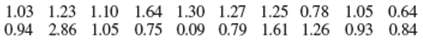
- a. Would you use the one-sample t test to decide whether there is compelling evidence for concluding that the population mean turnover is less than 100%? Explain.
- b. A normal
probability plot of the 20 ln(turnover) values shows a very pronounced linear pattern, suggesting it is reasonable to assume that the turnover distribution is lognormal. Recall that X has a lognormal distribution if In(X) isnormally distributed withmean value μ and variance σ2. Because μ, is also themedian of the ln(X) distribution, eμ is the median of the X distribution. Use this information to decide whether there is compelling evidence for concluding that the median of the turnover population distribution is less than 100%.
Expert Solution & Answer
Want to see the full answer?
Check out a sample textbook solution
Students have asked these similar questions
Selon une économiste d’une société financière, les dépenses moyennes pour « meubles et appareils de maison » ont été moins importantes pour les ménages de la région de Montréal, que celles de la région de Québec.
Un échantillon aléatoire de 14 ménages pour la région de Montréal et de 16 ménages pour la région Québec est tiré et donne les données suivantes, en ce qui a trait aux dépenses pour ce secteur d’activité économique.
On suppose que les données de chaque population sont distribuées selon une loi normale.
Nous sommes intéressé à connaitre si les variances des populations sont égales.a) Faites le test d’hypothèse sur deux variances approprié au seuil de signification de 1 %. Inclure les informations suivantes :
i. Hypothèse / Identification des populationsii. Valeur(s) critique(s) de Fiii. Règle de décisioniv. Valeur du rapport Fv. Décision et conclusion
b) A partir des résultats obtenus en a), est-ce que l’hypothèse d’égalité des variances pour cette…
According to an economist from a financial company, the average expenditures on "furniture and household appliances" have been lower for households in the Montreal area than those in the Quebec region.
A random sample of 14 households from the Montreal region and 16 households from the Quebec region was taken, providing the following data regarding expenditures in this economic sector.
It is assumed that the data from each population are distributed normally.
We are interested in knowing if the variances of the populations are equal. a) Perform the appropriate hypothesis test on two variances at a significance level of 1%. Include the following information:
i. Hypothesis / Identification of populations ii. Critical F-value(s) iii. Decision rule iv. F-ratio value v. Decision and conclusion
b) Based on the results obtained in a), is the hypothesis of equal variances for this socio-economic characteristic measured in these two populations upheld?
c) Based on the results obtained in a),…
A major company in the Montreal area, offering a range of engineering services from project preparation to construction execution, and industrial project management, wants to ensure that the individuals who are responsible for project cost estimation and bid preparation demonstrate a certain uniformity in their estimates. The head of civil engineering and municipal services decided to structure an experimental plan to detect if there could be significant differences in project evaluation.
Seven projects were selected, each of which had to be evaluated by each of the two estimators, with the order of the projects submitted being random. The obtained estimates are presented in the table below.
a) Complete the table above by calculating: i. The differences (A-B) ii. The sum of the differences iii. The mean of the differences iv. The standard deviation of the differences
b) What is the value of the t-statistic?
c) What is the critical t-value for this test at a significance level of 1%?…
Chapter 8 Solutions
Probability and Statistics for Engineering and the Sciences
Ch. 8.1 - For each of the following assertions, state...Ch. 8.1 - For the following pairs of assertions, indicate...Ch. 8.1 - For which of the given P-values would the null...Ch. 8.1 - Pairs of P-values and significance levels, , are...Ch. 8.1 - To determine whether the pipe welds in a nuclear...Ch. 8.1 - Let denote the true average radioactivity level...Ch. 8.1 - Before agreeing to purchase a large order of...Ch. 8.1 - Many older homes have electrical systems that use...Ch. 8.1 - Water samples are taken from water used for...Ch. 8.1 - A regular type of laminate is currently being used...
Ch. 8.1 - Prob. 11ECh. 8.1 - A mixture of pulverized fuel ash and Portland...Ch. 8.1 - The calibration of a scale is to be checked by...Ch. 8.1 - A new design for the braking system on a certain...Ch. 8.2 - Let denote the true average reaction time to a...Ch. 8.2 - Newly purchased tires of a particular type are...Ch. 8.2 - Answer the following questions for the tire...Ch. 8.2 - Reconsider the paint-drying situation of Example...Ch. 8.2 - The melting point of each of 16 samples of a...Ch. 8.2 - Lightbulbs of a certain type are advertised as...Ch. 8.2 - The desired percentage of SiO2 in a certain type...Ch. 8.2 - To obtain information on the corrosion-resistance...Ch. 8.2 - Automatic identification of the boundaries of...Ch. 8.2 - Unlike most packaged food products, alcohol...Ch. 8.2 - Body armor provides critical protection for law...Ch. 8.2 - Prob. 26ECh. 8.2 - Show that for any 0, when the population...Ch. 8.2 - For a fixed alternative value , show that () 0 as...Ch. 8.3 - The true average diameter of ball bearings of a...Ch. 8.3 - A sample of n sludge specimens is selected and the...Ch. 8.3 - The paint used to make lines on roads must reflect...Ch. 8.3 - The relative conductivity of a semiconductor...Ch. 8.3 - The article The Foremans View of Quality Control...Ch. 8.3 - The following observations are on stopping...Ch. 8.3 - The article Uncertainty Estimation in Railway...Ch. 8.3 - Have you ever been frustrated because you could...Ch. 8.3 - The accompanying data on cube compressive strength...Ch. 8.3 - A random sample of soil specimens was obtained,...Ch. 8.3 - Reconsider the accompanying sample data on expense...Ch. 8.3 - Polymer composite materials have gained popularity...Ch. 8.3 - A spectrophotometer used for measuring CO...Ch. 8.4 - Prob. 42ECh. 8.4 - Prob. 43ECh. 8.4 - A manufacturer of nickel-hydrogen batteries...Ch. 8.4 - A random sample of 150 recent donations at a...Ch. 8.4 - It is known that roughly 2/3 of all human beings...Ch. 8.4 - The article Effects of Bottle Closure Type on...Ch. 8.4 - With domestic sources of building supplies running...Ch. 8.4 - A plan for an executive travelers club has been...Ch. 8.4 - Each of a group of 20 intermediate tennis players...Ch. 8.4 - A manufacturer of plumbing fixtures has developed...Ch. 8.4 - In a sample of 171 students at an Australian...Ch. 8.5 - Reconsider the paint-drying problem discussed in...Ch. 8.5 - Consider the large-sample level .01 test in...Ch. 8.5 - Consider carrying out m tests of hypotheses based...Ch. 8.5 - Prob. 56ECh. 8 - A sample of 50 lenses used in eyeglasses yields a...Ch. 8 - In Exercise 57, suppose the experimenter had...Ch. 8 - It is specified that a certain type of iron should...Ch. 8 - One method for straightening wire before coiling...Ch. 8 - Contamination of mine soils in China is a serious...Ch. 8 - The article Orchard Floor Management Utilizing...Ch. 8 - The article Caffeine Knowledge, Attitudes, and...Ch. 8 - Annual holdings turnover for a mutual fund is the...Ch. 8 - The true average breaking strength of ceramic...Ch. 8 - Prob. 66SECh. 8 - The incidence of a certain type of chromosome...Ch. 8 - Prob. 68SECh. 8 - Prob. 69SECh. 8 - The Dec. 30, 2009. the New York Times reported...Ch. 8 - When X1, X2,, Xn are independent Poisson...Ch. 8 - An article in the Nov. 11, 2005, issue of the San...Ch. 8 - Prob. 73SECh. 8 - The article Analysis of Reserve and Regular...Ch. 8 - Prob. 75SECh. 8 - Chapter 7 presented a CI for the variance 2 of a...Ch. 8 - Prob. 77SECh. 8 - When the population distribution is normal and n...Ch. 8 - Let X1, X2, Xn be a random sample from an...Ch. 8 - Because of variability in the manufacturing...
Knowledge Booster


Learn more about
Need a deep-dive on the concept behind this application? Look no further. Learn more about this topic, statistics and related others by exploring similar questions and additional content below.Similar questions
- Compute the relative risk of falling for the two groups (did not stop walking vs. did stop). State/interpret your result verbally.arrow_forwardMicrosoft Excel include formulasarrow_forwardQuestion 1 The data shown in Table 1 are and R values for 24 samples of size n = 5 taken from a process producing bearings. The measurements are made on the inside diameter of the bearing, with only the last three decimals recorded (i.e., 34.5 should be 0.50345). Table 1: Bearing Diameter Data Sample Number I R Sample Number I R 1 34.5 3 13 35.4 8 2 34.2 4 14 34.0 6 3 31.6 4 15 37.1 5 4 31.5 4 16 34.9 7 5 35.0 5 17 33.5 4 6 34.1 6 18 31.7 3 7 32.6 4 19 34.0 8 8 33.8 3 20 35.1 9 34.8 7 21 33.7 2 10 33.6 8 22 32.8 1 11 31.9 3 23 33.5 3 12 38.6 9 24 34.2 2 (a) Set up and R charts on this process. Does the process seem to be in statistical control? If necessary, revise the trial control limits. [15 pts] (b) If specifications on this diameter are 0.5030±0.0010, find the percentage of nonconforming bearings pro- duced by this process. Assume that diameter is normally distributed. [10 pts] 1arrow_forward
- 4. (5 pts) Conduct a chi-square contingency test (test of independence) to assess whether there is an association between the behavior of the elderly person (did not stop to talk, did stop to talk) and their likelihood of falling. Below, please state your null and alternative hypotheses, calculate your expected values and write them in the table, compute the test statistic, test the null by comparing your test statistic to the critical value in Table A (p. 713-714) of your textbook and/or estimating the P-value, and provide your conclusions in written form. Make sure to show your work. Did not stop walking to talk Stopped walking to talk Suffered a fall 12 11 Totals 23 Did not suffer a fall | 2 Totals 35 37 14 46 60 Tarrow_forwardQuestion 2 Parts manufactured by an injection molding process are subjected to a compressive strength test. Twenty samples of five parts each are collected, and the compressive strengths (in psi) are shown in Table 2. Table 2: Strength Data for Question 2 Sample Number x1 x2 23 x4 x5 R 1 83.0 2 88.6 78.3 78.8 3 85.7 75.8 84.3 81.2 78.7 75.7 77.0 71.0 84.2 81.0 79.1 7.3 80.2 17.6 75.2 80.4 10.4 4 80.8 74.4 82.5 74.1 75.7 77.5 8.4 5 83.4 78.4 82.6 78.2 78.9 80.3 5.2 File Preview 6 75.3 79.9 87.3 89.7 81.8 82.8 14.5 7 74.5 78.0 80.8 73.4 79.7 77.3 7.4 8 79.2 84.4 81.5 86.0 74.5 81.1 11.4 9 80.5 86.2 76.2 64.1 80.2 81.4 9.9 10 75.7 75.2 71.1 82.1 74.3 75.7 10.9 11 80.0 81.5 78.4 73.8 78.1 78.4 7.7 12 80.6 81.8 79.3 73.8 81.7 79.4 8.0 13 82.7 81.3 79.1 82.0 79.5 80.9 3.6 14 79.2 74.9 78.6 77.7 75.3 77.1 4.3 15 85.5 82.1 82.8 73.4 71.7 79.1 13.8 16 78.8 79.6 80.2 79.1 80.8 79.7 2.0 17 82.1 78.2 18 84.5 76.9 75.5 83.5 81.2 19 79.0 77.8 20 84.5 73.1 78.2 82.1 79.2 81.1 7.6 81.2 84.4 81.6 80.8…arrow_forwardName: Lab Time: Quiz 7 & 8 (Take Home) - due Wednesday, Feb. 26 Contingency Analysis (Ch. 9) In lab 5, part 3, you will create a mosaic plot and conducted a chi-square contingency test to evaluate whether elderly patients who did not stop walking to talk (vs. those who did stop) were more likely to suffer a fall in the next six months. I have tabulated the data below. Answer the questions below. Please show your calculations on this or a separate sheet. Did not stop walking to talk Stopped walking to talk Totals Suffered a fall Did not suffer a fall Totals 12 11 23 2 35 37 14 14 46 60 Quiz 7: 1. (2 pts) Compute the odds of falling for each group. Compute the odds ratio for those who did not stop walking vs. those who did stop walking. Interpret your result verbally.arrow_forward
- Solve please and thank you!arrow_forward7. In a 2011 article, M. Radelet and G. Pierce reported a logistic prediction equation for the death penalty verdicts in North Carolina. Let Y denote whether a subject convicted of murder received the death penalty (1=yes), for the defendant's race h (h1, black; h = 2, white), victim's race i (i = 1, black; i = 2, white), and number of additional factors j (j = 0, 1, 2). For the model logit[P(Y = 1)] = a + ß₁₂ + By + B²², they reported = -5.26, D â BD = 0, BD = 0.17, BY = 0, BY = 0.91, B = 0, B = 2.02, B = 3.98. (a) Estimate the probability of receiving the death penalty for the group most likely to receive it. [4 pts] (b) If, instead, parameters used constraints 3D = BY = 35 = 0, report the esti- mates. [3 pts] h (c) If, instead, parameters used constraints Σ₁ = Σ₁ BY = Σ; B = 0, report the estimates. [3 pts] Hint the probabilities, odds and odds ratios do not change with constraints.arrow_forwardSolve please and thank you!arrow_forward
- Solve please and thank you!arrow_forwardQuestion 1:We want to evaluate the impact on the monetary economy for a company of two types of strategy (competitive strategy, cooperative strategy) adopted by buyers.Competitive strategy: strategy characterized by firm behavior aimed at obtaining concessions from the buyer.Cooperative strategy: a strategy based on a problem-solving negotiating attitude, with a high level of trust and cooperation.A random sample of 17 buyers took part in a negotiation experiment in which 9 buyers adopted the competitive strategy, and the other 8 the cooperative strategy. The savings obtained for each group of buyers are presented in the pdf that i sent: For this problem, we assume that the samples are random and come from two normal populations of unknown but equal variances.According to the theory, the average saving of buyers adopting a competitive strategy will be lower than that of buyers adopting a cooperative strategy.a) Specify the population identifications and the hypotheses H0 and H1…arrow_forwardYou assume that the annual incomes for certain workers are normal with a mean of $28,500 and a standard deviation of $2,400. What’s the chance that a randomly selected employee makes more than $30,000?What’s the chance that 36 randomly selected employees make more than $30,000, on average?arrow_forward
arrow_back_ios
SEE MORE QUESTIONS
arrow_forward_ios
Recommended textbooks for you
 Linear Algebra: A Modern IntroductionAlgebraISBN:9781285463247Author:David PoolePublisher:Cengage Learning
 Big Ideas Math A Bridge To Success Algebra 1: Stu...AlgebraISBN:9781680331141Author:HOUGHTON MIFFLIN HARCOURTPublisher:Houghton Mifflin Harcourt
Linear Algebra: A Modern Introduction
Algebra
ISBN:9781285463247
Author:David Poole
Publisher:Cengage Learning
Big Ideas Math A Bridge To Success Algebra 1: Stu...
Algebra
ISBN:9781680331141
Author:HOUGHTON MIFFLIN HARCOURT
Publisher:Houghton Mifflin Harcourt
Introduction to experimental design and analysis of variance (ANOVA); Author: Dr. Bharatendra Rai;https://www.youtube.com/watch?v=vSFo1MwLoxU;License: Standard YouTube License, CC-BY