Subpart (a):
Equilibrium price .
Subpart (a):
Explanation of Solution
The equilibrium
We have given the supply equation and the demand equations and we can equate them in order to obtain the equilibrium price as follows:
Thus, the equilibrium price is $100. Now we can calculate the equilibrium quantity by substituting the equilibrium price in the equations as follows:
Thus, the equilibrium quantity is 200 units.
Concept introduction:
Equilibrium: It is the
Subpart (b):
Equilibrium price.
Subpart (b):
Explanation of Solution
We have given the supply equation and the demand equation changes due to the tax on consumers and the new demand equation is
Thus, the price received by the producers is
Thus, the quantity is now
Concept introduction:
Equilibrium: It is the market equilibrium which is determined by equating the supply to the demand. At this equilibrium point, the supply will be equal to the demand and there will be no excess demand or excess supply in the economy. Thus, the economy will be at equilibrium.
Subpart (c):
Total tax revenue.
Subpart (c):
Explanation of Solution
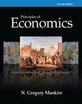
We have given that the tax revenue equals to the tax rate multiplied with the quantity. The quantity is calculated in part b as
This relation between the tax revenue can be illustrated as follows:
The graph depicts that the tax revenue will be zero at the tax levels of T = $0 and also at the tax rate of T = $300.
Concept introduction:
Tax: It is the unilateral payment made by the public towards the government. There are many different types of taxes in the economy which include the income tax, property tax and professional tax and so forth.
Tax revenue: Tax revenue refers to the total revenue earned by the government through imposing tax.
Subpart (d):
Deadweight loss .
Subpart (d):
Explanation of Solution
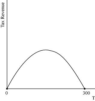
We have given that deadweight loss is the area of the triangle between the demand and supply curves. The following diagram shows, the area of the triangle (laid on its side) that represents the deadweight loss is 1/2 × base × height, where the base is the change in the price, which is the size of the tax (T) and the height is the amount of the decline in quantity (
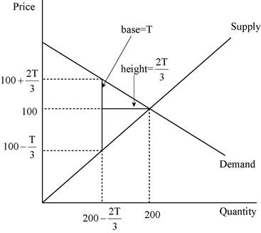
The deadweight loss can be calculated as follows:
Thus, the deadweight loss is equal to
In the above diagram horizontal axis measures quantity and vertical axis measures deadweight loss.
Concept introduction:
Tax: It is the unilateral payment made by the public towards the government. There are many different types of taxes in the economy which include the income tax, property tax and professional tax and so forth.
Deadweight loss: It is the reduction in the units where the marginal benefit to the consumer is higher than the marginal cost of production of the unit.
Subpart (e):
Determine the tax amount.
Subpart (e):
Explanation of Solution
A tax of $200 will not turn out to be a good policy because the tax revenue decreases when the tax rate reaches to $300 where the tax revenue is zero. The tax revenue is at its maximum at the middle of the tax rate of $0 and $300 which is $150. Thus, in order to increase the tax revenue, the government should reduce the tax rate to $150 from $200 which will be the good alternative policy.
Concept introduction:
Tax: It is the unilateral payment made by the public towards the government. There are many different types of taxes in the economy which include the income tax, property tax and professional tax and so forth.
Want to see more full solutions like this?
Chapter 8 Solutions
EBK PRINCIPLES OF ECONOMICS

- Title: Does the educational performance depend on its literacy rate and government spending over the last 10 years? In the introduction, there are four things to include:a) Clearly state your research topic follows by country’s background in terms of (population density; male/female ratio; and identify the problem leading up to the study of it, such as government spending and adult literacy rate. How does the US perform compared to other countries.b) State the research question that you wish to resolve: Does the US economic performance depend on its government spending on education and the literacy rate over the last 10 years. Define performance (Y) as the average income per capita, an indicator of the country’s economy growing over time. For example, an increase in government spending leads to higher literacy rates and subsequently higher productivity in the economy. Also, mention that you will use a sample size of 10 years of secondary data from the existing literature,…arrow_forwardTitle: Does the educational performance depend on its literacy rate and government spending over the last 10 years? In the introduction, there are four things to include:a) Clearly state your research topic follows by country’s background in terms of (population density; male/female ratio; and identify the problem leading up to the study of it, such as government spending and adult literacy rate. How does the US perform compared to other countries.b) State the research question that you wish to resolve: Does the US economic performance depend on its government spending on education and the literacy rate over the last 10 years. Define performance (Y) as the average income per capita, an indicator of the country’s economy growing over time. For example, an increase in government spending leads to higher literacy rates and subsequently higher productivity in the economy. Also, mention that you will use a sample size of 10 years of secondary data from the existing literature,…arrow_forwardExplain how the introduction of egg replacers and plant-based egg products will impact the bakery industry. Provide a graphical representation.arrow_forward
- Explain Professor Frederick's "cognitive reflection" test.arrow_forward11:44 Fri Apr 4 Would+You+Take+the+Bird+in+the+Hand Would You Take the Bird in the Hand, or a 75% Chance at the Two in the Bush? BY VIRGINIA POSTREL WOULD you rather have $1,000 for sure or a 90 percent chance of $5,000? A guaranteed $1,000 or a 75 percent chance of $4,000? In economic theory, questions like these have no right or wrong answers. Even if a gamble is mathematically more valuable a 75 percent chance of $4,000 has an expected value of $3,000, for instance someone may still prefer a sure thing. People have different tastes for risk, just as they have different tastes for ice cream or paint colors. The same is true for waiting: Would you rather have $400 now or $100 every year for 10 years? How about $3,400 this month or $3,800 next month? Different people will answer differently. Economists generally accept those differences without further explanation, while decision researchers tend to focus on average behavior. In decision research, individual differences "are regarded…arrow_forwardDescribe the various measures used to assess poverty and economic inequality. Analyze the causes and consequences of poverty and inequality, and discuss potential policies and programs aimed at reducing them, assess the adequacy of current environmental regulations in addressing negative externalities. analyze the role of labor unions in labor markets. What is one benefit, and one challenge associated with labor unions.arrow_forward
- Evaluate the effectiveness of supply and demand models in predicting labor market outcomes. Justify your assessment with specific examples from real-world labor markets.arrow_forwardExplain the difference between Microeconomics and Macroeconomics? 2.) Explain what fiscal policy is and then explain what Monetary Policy is? 3.) Why is opportunity cost and give one example from your own of opportunity cost. 4.) What are models and what model did we already discuss in class? 5.) What is meant by scarcity of resources?arrow_forward2. What is the payoff from a long futures position where you are obligated to buy at the contract price? What is the payoff from a short futures position where you are obligated to sell at the contract price?? Draw the payoff diagram for each position. Payoff from Futures Contract F=$50.85 S1 Long $100 $95 $90 $85 $80 $75 $70 $65 $60 $55 $50.85 $50 $45 $40 $35 $30 $25 Shortarrow_forward
- 3. Consider a call on the same underlier (Cisco). The strike is $50.85, which is the forward price. The owner of the call has the choice or option to buy at the strike. They get to see the market price S1 before they decide. We assume they are rational. What is the payoff from owning (also known as being long) the call? What is the payoff from selling (also known as being short) the call? Payoff from Call with Strike of k=$50.85 S1 Long $100 $95 $90 $85 $80 $75 $70 $65 $60 $55 $50.85 $50 $45 $40 $35 $30 $25 Shortarrow_forward4. Consider a put on the same underlier (Cisco). The strike is $50.85, which is the forward price. The owner of the call has the choice or option to buy at the strike. They get to see the market price S1 before they decide. We assume they are rational. What is the payoff from owning (also known as being long) the put? What is the payoff from selling (also known as being short) the put? Payoff from Put with Strike of k=$50.85 S1 Long $100 $95 $90 $85 $80 $75 $70 $65 $60 $55 $50.85 $50 $45 $40 $35 $30 $25 Shortarrow_forwardThe following table provides information on two technology companies, IBM and Cisco. Use the data to answer the following questions. Company IBM Cisco Systems Stock Price Dividend (trailing 12 months) $150.00 $50.00 $7.00 Dividend (next 12 months) $7.35 Dividend Growth 5.0% $2.00 $2.15 7.5% 1. You buy a futures contract instead of purchasing Cisco stock at $50. What is the one-year futures price, assuming the risk-free interest rate is 6%? Remember to adjust the futures price for the dividend of $2.15.arrow_forward
 Microeconomics: Principles & PolicyEconomicsISBN:9781337794992Author:William J. Baumol, Alan S. Blinder, John L. SolowPublisher:Cengage Learning


