
Subpart (a):
Subpart (a):
Explanation of Solution
The equilibrium
We have given the supply equation and the demand equations and we can equate them in order to obtain the equilibrium price as follows:
Thus, the equilibrium price is $100. Now we can calculate the equilibrium quantity by substituting the equilibrium price in the equations as follows:
Thus, the equilibrium quantity is 200 units.
Concept introduction:
Equilibrium: It is the
Subpart (b):
Equilibrium price.
Subpart (b):
Explanation of Solution
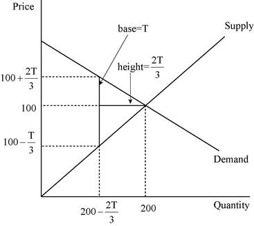
We have given the supply equation and the demand equation changes due to the tax on consumers and the new demand equation is
Thus, the price received by the producers is
Thus, the quantity is now
Concept introduction:
Equilibrium: It is the market equilibrium which is determined by equating the supply to the demand. At this equilibrium point, the supply will be equal to the demand and there will be no excess demand or excess supply in the economy. Thus, the economy will be at equilibrium.
Subpart (c):
Total tax revenue.
Subpart (c):
Explanation of Solution
We have given that the tax revenue equals to the tax rate multiplied with the quantity. The quantity is calculated in part b as
This relation between the tax revenue can be illustrated as follows:
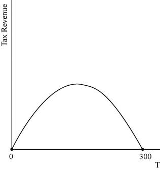
The graph depicts that the tax revenue will be zero at the tax levels of T = $0 and also at the tax rate of T = $300.
Concept introduction:
Tax: It is the unilateral payment made by the public towards the government. There are many different types of taxes in the economy which include the income tax, property tax and professional tax and so forth.
Tax revenue: Tax revenue refers to the total revenue earned by the government through imposing tax.
Subpart (d):
Subpart (d):
Explanation of Solution
We have given that deadweight loss is the area of the triangle between the demand and supply curves. The following diagram shows, the area of the triangle (laid on its side) that represents the deadweight loss is 1/2 × base × height, where the base is the change in the price, which is the size of the tax (T) and the height is the amount of the decline in quantity (
The deadweight loss can be calculated as follows:
Thus, the deadweight loss is equal to
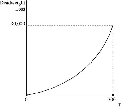
In the above diagram horizontal axis measures quantity and vertical axis measures deadweight loss.
Concept introduction:
Tax: It is the unilateral payment made by the public towards the government. There are many different types of taxes in the economy which include the income tax, property tax and professional tax and so forth.
Deadweight loss: It is the reduction in the units where the marginal benefit to the consumer is higher than the marginal cost of production of the unit.
Subpart (e):
Determine the tax amount.
Subpart (e):
Explanation of Solution
A tax of $200 will not turn out to be a good policy because the tax revenue decreases when the tax rate reaches to $300 where the tax revenue is zero. The tax revenue is at its maximum at the middle of the tax rate of $0 and $300 which is $150. Thus, in order to increase the tax revenue, the government should reduce the tax rate to $150 from $200 which will be the good alternative policy.
Concept introduction:
Tax: It is the unilateral payment made by the public towards the government. There are many different types of taxes in the economy which include the income tax, property tax and professional tax and so forth.
Want to see more full solutions like this?
Chapter 8 Solutions
Bundle: Essentials Of Economics, Loose-leaf Version, 8th + Lms Integrated Mindtap Economics, 1 Term (6 Months) Printed Access Card

- 19. In a paragraph, no bullet, points please answer the question and follow the instructions. Give only the solution: Use the Feynman technique throughout. Assume that you’re explaining the answer to someone who doesn’t know the topic at all. How does the Federal Reserve currently get the federal funds rate where they want it to be?arrow_forward18. In a paragraph, no bullet, points please answer the question and follow the instructions. Give only the solution: Use the Feynman technique throughout. Assume that you’re explaining the answer to someone who doesn’t know the topic at all. Carefully compare and contrast fiscal policy and monetary policy.arrow_forward15. In a paragraph, no bullet, points please answer the question and follow the instructions. Give only the solution: Use the Feynman technique throughout. Assume that you’re explaining the answer to someone who doesn’t know the topic at all. What are the common arguments for and against high levels of federal debt?arrow_forward
- 17. In a paragraph, no bullet, points please answer the question and follow the instructions. Give only the solution: Use the Feynman technique throughout. Assume that you’re explaining the answer to someone who doesn’t know the topic at all. Explain the difference between present value and future value. Be sure to use and explain the mathematical formulas for both. How does one interpret these formulas?arrow_forward12. Give the solution: Use the Feynman technique throughout. Assume that you’re explaining the answer to someone who doesn’t know the topic at all. Show and carefully explain the Taylor rule and all of its components, used as a monetary policy guide.arrow_forward20. In a paragraph, no bullet, points please answer the question and follow the instructions. Give only the solution: Use the Feynman technique throughout. Assume that you’re explaining the answer to someone who doesn’t know the topic at all. What is meant by the Federal Reserve’s new term “ample reserves”? What may be hidden in this new formulation by the Fed?arrow_forward
- 14. In a paragraph, no bullet, points please answer the question and follow the instructions. Give only the solution: Use the Feynman technique throughout. Assume that you’re explaining the answer to someone who doesn’t know the topic at all. What is the Keynesian view of fiscal policy and why are some economists skeptical?arrow_forward16. In a paragraph, no bullet, points please answer the question and follow the instructions. Give only the solution: Use the Feynman technique throughout. Assume that you’re explaining the answer to someone who doesn’t know the topic at all. Describe a bond or Treasury security. What are its components and what do they mean?arrow_forward13. In a paragraph, no bullet, points please answer the question and follow the instructions. Give only the solution: Use the Feynman technique throughout. Assume that you’re explaining the answer to someone who doesn’t know the topic at all. Where does the government get its funds that it spends? What is the difference between federal debt and federal deficit?arrow_forward
- 11. In a paragraph, no bullet, points please answer the question and follow the instructions. Give only the solution: Use the Feynman technique throughout. Assume that you’re explaining the answer to someone who doesn’t know the topic at all. Why is determining the precise interest rate target so difficult for the Fed?arrow_forwardProblem 1 Regression Discontinuity In the beginning of covid, the US government distributed covid stimulus payments. Suppose you are interested in the effect of receiving the full amount of the first stimulus payment on the total spending in dollars by single individuals in the month after receiving the payment. Single individuals with annual income below $75,00 received the full amount of the stimulus payment. You decide to use Regression Discontinuity to answer this question. The graph below shows the RD model. 3150 3100 3050 Total Spending in the month after receiving the stimulus payment 2950 3000 74000 74500 75000 75500 76000 Annual income a. What is the outcome? (5 points) b. What is the treatment? (5 points) C. What is the running variable? (5 points) d. What is the cutoff? (5 points) e. Who is in the treatment group and who is in the control group? (10 points) f. What is the discontinuity in the graph and how do you interpret it? (10 points) g. Explain a scenario which can…arrow_forwardProblem 2 Difference-in-Difference In the beginning of 2005, Minnesota increased the sales tax on alcohol. Suppose you are interested in studying the effect of the increase in sale taxes on alcohol on the number of car accidents due to drinking in Minnesota. Unlike Minnesota, Wisconsin did not change the sales tax on alcohol. You decide to use a Difference-in-difference (DID) Model. The numbers of car accidents in each state at the end of 2004 and 2005 are as follows: Year Number of car accidents in Minnesota Number of car accidents in Wisconsin 2004 2000 2500 2005 2500 3500 a. Which state is the treatment state and which state is the control state? (10 points) b. What is the change in the outcome for the treatment group between 2004 and 2005? (5 points) C. Can we interpret the change in the outcome for the treatment group between 2004 and 2005 as the causal effect of the policy on car accidents? Explain your answer. (10 points) d. What is the change in the outcome for the control…arrow_forward
 Microeconomics: Principles & PolicyEconomicsISBN:9781337794992Author:William J. Baumol, Alan S. Blinder, John L. SolowPublisher:Cengage Learning


