
Concept explainers
Videos
a.
Find the exact and approximate values of
a.
Answer to Problem 67E
The exact and approximate values of
The exact and approximate values of
The exact and approximate values of
The exact and approximate values of
Explanation of Solution
From the given information, Y follows binomial distribution and
For
Step-by-step procedure to obtain the probability using APPLET:
- Choose Normal approximation to binomial distribution under Applets.
- Set the n value as 5 and p value as 0.20.
- Select the bars 0 and 4.
Output using APPLET is given below:
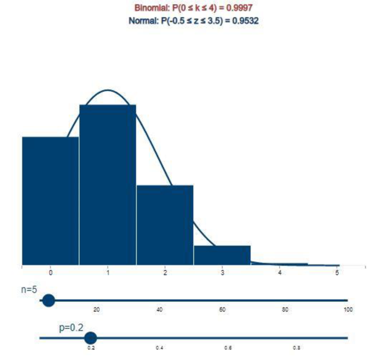
From the above output, it can be observed that exact and approximate values are 0.9997 and 0.9532, respectively.
Thus, the exact and approximate values of
For
Step-by-step procedure to obtain the probability using APPLET:
- Choose Normal approximation to binomial distribution under Applets.
- Set the n value as 10 and p value as 0.20.
- Select the bars 0 and 5.
Output using APPLET is given below:
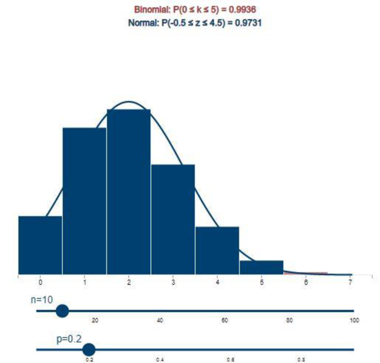
From the above output, it can be observed that exact and approximate values are 0.9936 and 0.9731, respectively.
Thus, the exact and approximate values of
For
Step-by-step procedure to obtain the probability using APPLET:
- Choose Normal approximation to binomial distribution under Applets.
- Set the n value as 15 and p value as 0.20.
- Select the bars 0 and 6.
Output using APPLET is given below:
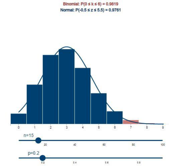
From the above output, it can be observed that exact and approximate values are 0.9819 and 0.9761, respectively.
Thus, the exact and approximate values of
For
Step-by-step procedure to obtain the probability using APPLET:
- Choose Normal approximation to binomial distribution under Applets.
- Set the n value as 20 and p value as 0.20.
- Select the bars 0 and 7.
Output using APPLET is given below:
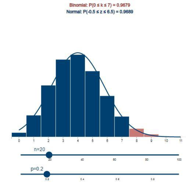
From the above output, it can be observed that exact and approximate values are 0.9679 and 0.9689, respectively.
Thus, the exact and approximate values of
b.
Give the observation about the shapes of the binomial histograms as the
Give the observation about the differences between the exact and approximate values of
b.
Answer to Problem 67E
The observation is that the shapes of the binomial histograms tend to bell shaped by increasing the sample size.
The difference between the exact and approximate values of
Explanation of Solution
From the histograms in part a, it can be observed that as the sample size increases the binomial histograms become bell shaped.
Thus, the observation is that the shapes of the binomial histograms tend to bell shaped by increasing the sample size.
From the part a, it can be observed that
The exact and approximate values of
The exact and approximate values of
The exact and approximate values of
The exact and approximate values of
From the above results it can be observed that as the sample size increases the difference between the exact and approximate values of
Thus, the difference between the exact and approximate values of
c.
Find the sample size n for the approximation to be adequate.
Check whether this is consistent with that observed in parts (a) and (b).
c.
Answer to Problem 67E
The sample size n for the approximation to be adequate is 36.
The sample size is consistent with that observed in parts (a) and (b).
Explanation of Solution
It is known that, the normal approximate to the binomial approximation is adequate if
From the given information,
Then,
Thus, the sample size n for the approximation to be adequate is 36.
From the parts a and b it can be observed that as the sample size increases the exact and approximate values of
Thus, the sample size is consistent with that observed in parts (a) and (b).
Want to see more full solutions like this?
Chapter 7 Solutions
Mathematical Statistics with Applications


- Question: A company launches two different marketing campaigns to promote the same product in two different regions. After one month, the company collects the sales data (in units sold) from both regions to compare the effectiveness of the campaigns. The company wants to determine whether there is a significant difference in the mean sales between the two regions. Perform a two sample T-test You can provide your answer by inserting a text box and the answer must include: Null hypothesis, Alternative hypothesis, Show answer (output table/summary table), and Conclusion based on the P value. (2 points = 0.5 x 4 Answers) Each of these is worth 0.5 points. However, showing the calculation is must. If calculation is missing, the whole answer won't get any credit.arrow_forwardBinomial Prob. Question: A new teaching method claims to improve student engagement. A survey reveals that 60% of students find this method engaging. If 15 students are randomly selected, what is the probability that: a) Exactly 9 students find the method engaging?b) At least 7 students find the method engaging? (2 points = 1 x 2 answers) Provide answers in the yellow cellsarrow_forwardIn a survey of 2273 adults, 739 say they believe in UFOS. Construct a 95% confidence interval for the population proportion of adults who believe in UFOs. A 95% confidence interval for the population proportion is ( ☐, ☐ ). (Round to three decimal places as needed.)arrow_forward
- Find the minimum sample size n needed to estimate μ for the given values of c, σ, and E. C=0.98, σ 6.7, and E = 2 Assume that a preliminary sample has at least 30 members. n = (Round up to the nearest whole number.)arrow_forwardIn a survey of 2193 adults in a recent year, 1233 say they have made a New Year's resolution. Construct 90% and 95% confidence intervals for the population proportion. Interpret the results and compare the widths of the confidence intervals. The 90% confidence interval for the population proportion p is (Round to three decimal places as needed.) J.D) .arrow_forwardLet p be the population proportion for the following condition. Find the point estimates for p and q. In a survey of 1143 adults from country A, 317 said that they were not confident that the food they eat in country A is safe. The point estimate for p, p, is (Round to three decimal places as needed.) ...arrow_forward
- (c) Because logistic regression predicts probabilities of outcomes, observations used to build a logistic regression model need not be independent. A. false: all observations must be independent B. true C. false: only observations with the same outcome need to be independent I ANSWERED: A. false: all observations must be independent. (This was marked wrong but I have no idea why. Isn't this a basic assumption of logistic regression)arrow_forwardBusiness discussarrow_forwardSpam filters are built on principles similar to those used in logistic regression. We fit a probability that each message is spam or not spam. We have several variables for each email. Here are a few: to_multiple=1 if there are multiple recipients, winner=1 if the word 'winner' appears in the subject line, format=1 if the email is poorly formatted, re_subj=1 if "re" appears in the subject line. A logistic model was fit to a dataset with the following output: Estimate SE Z Pr(>|Z|) (Intercept) -0.8161 0.086 -9.4895 0 to_multiple -2.5651 0.3052 -8.4047 0 winner 1.5801 0.3156 5.0067 0 format -0.1528 0.1136 -1.3451 0.1786 re_subj -2.8401 0.363 -7.824 0 (a) Write down the model using the coefficients from the model fit.log_odds(spam) = -0.8161 + -2.5651 + to_multiple + 1.5801 winner + -0.1528 format + -2.8401 re_subj(b) Suppose we have an observation where to_multiple=0, winner=1, format=0, and re_subj=0. What is the predicted probability that this message is spam?…arrow_forward
- Consider an event X comprised of three outcomes whose probabilities are 9/18, 1/18,and 6/18. Compute the probability of the complement of the event. Question content area bottom Part 1 A.1/2 B.2/18 C.16/18 D.16/3arrow_forwardJohn and Mike were offered mints. What is the probability that at least John or Mike would respond favorably? (Hint: Use the classical definition.) Question content area bottom Part 1 A.1/2 B.3/4 C.1/8 D.3/8arrow_forwardThe details of the clock sales at a supermarket for the past 6 weeks are shown in the table below. The time series appears to be relatively stable, without trend, seasonal, or cyclical effects. The simple moving average value of k is set at 2. What is the simple moving average root mean square error? Round to two decimal places. Week Units sold 1 88 2 44 3 54 4 65 5 72 6 85 Question content area bottom Part 1 A. 207.13 B. 20.12 C. 14.39 D. 0.21arrow_forward
 Glencoe Algebra 1, Student Edition, 9780079039897...AlgebraISBN:9780079039897Author:CarterPublisher:McGraw Hill