
Statistics for Engineers and Scientists
4th Edition
ISBN: 9780073401331
Author: William Navidi Prof.
Publisher: McGraw-Hill Education
expand_more
expand_more
format_list_bulleted
Concept explainers
Videos
Textbook Question
Chapter 7.4, Problem 1E
The following output (from MINITAB) is for the least-squares fit of the model ln y = β0 + β1 ln x + ε, where y represents the monthly production of a gas well and x represents the volume of fracture fluid pumped in. (A
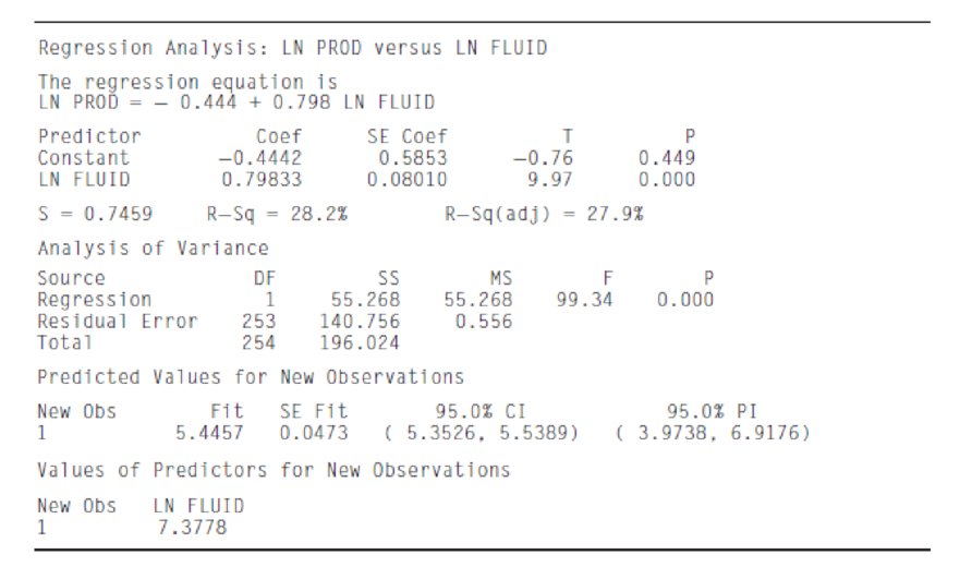
- a. What is the equation of the least-squares line for predicting ln y from ln x?
- b. Predict the production of a well into which 2500 gal/ft of fluid have been pumped.
- c. Predict the production of a well into which 1600 gal/ft of fluid have been pumped.
- d. Find a 95% prediction interval for the production of a well into which 1600 gal/ft of fluid have been pumped. (Note: In 1600 = 7.3778.)
Expert Solution & Answer
Want to see the full answer?
Check out a sample textbook solution
Students have asked these similar questions
NC Current Students - North Ce X | NC Canvas Login Links - North ( X
Final Exam Comprehensive x Cengage Learning
x
WASTAT - Final Exam - STAT
→
C
webassign.net/web/Student/Assignment-Responses/submit?dep=36055360&tags=autosave#question3659890_9
Part (b)
Draw a scatter plot of the ordered pairs.
N
Life
Expectancy
Life
Expectancy
80
70
600
50
40
30
20
10
Year of
1950
1970 1990
2010 Birth
O
Life
Expectancy
Part (c)
800
70
60
50
40
30
20
10
1950
1970 1990
W
ALT
林
$
#
4
R
J7
Year of
2010 Birth
F6
4+
80
70
60
50
40
30
20
10
Year of
1950 1970 1990
2010 Birth
Life
Expectancy
Ox
800
70
60
50
40
30
20
10
Year of
1950 1970 1990 2010 Birth
hp
P.B.
KA
&
7
80
% 5
H
A
B
F10
711
N
M
K
744
PRT SC
ALT
CTRL
Harvard University
California Institute of Technology
Massachusetts Institute of Technology
Stanford University
Princeton University
University of Cambridge
University of Oxford
University of California, Berkeley
Imperial College London
Yale University
University of California, Los Angeles
University of Chicago
Johns Hopkins University
Cornell University
ETH Zurich
University of Michigan
University of Toronto
Columbia University
University of Pennsylvania
Carnegie Mellon University
University of Hong Kong
University College London
University of Washington
Duke University
Northwestern University
University of Tokyo
Georgia Institute of Technology
Pohang University of Science and Technology
University of California, Santa Barbara
University of British Columbia
University of North Carolina at Chapel Hill
University of California, San Diego
University of Illinois at Urbana-Champaign
National University of Singapore
McGill…
Name
Harvard University
California Institute of Technology
Massachusetts Institute of Technology
Stanford University
Princeton University
University of Cambridge
University of Oxford
University of California, Berkeley
Imperial College London
Yale University
University of California, Los Angeles
University of Chicago
Johns Hopkins University
Cornell University
ETH Zurich
University of Michigan
University of Toronto
Columbia University
University of Pennsylvania
Carnegie Mellon University
University of Hong Kong
University College London
University of Washington
Duke University
Northwestern University
University of Tokyo
Georgia Institute of Technology
Pohang University of Science and Technology
University of California, Santa Barbara
University of British Columbia
University of North Carolina at Chapel Hill
University of California, San Diego
University of Illinois at Urbana-Champaign
National University of Singapore…
Chapter 7 Solutions
Statistics for Engineers and Scientists
Ch. 7.1 - Compute the correlation coefficient for the...Ch. 7.1 - For each of the following data sets, explain why...Ch. 7.1 - For each of the following scatterplots, state...Ch. 7.1 - True or false, and explain briefly: a. If the...Ch. 7.1 - In a study of ground motion caused by earthquakes,...Ch. 7.1 - A chemical engineer is studying the effect of...Ch. 7.1 - Another chemical engineer is studying the same...Ch. 7.1 - Tire pressure (in kPa) was measured for the right...Ch. 7.1 - Prob. 10ECh. 7.1 - The article Drift in Posturography Systems...
Ch. 7.1 - Prob. 12ECh. 7.1 - Prob. 13ECh. 7.1 - A scatterplot contains four points: (2, 2), (1,...Ch. 7.2 - Each month for several months, the average...Ch. 7.2 - In a study of the relationship between the Brinell...Ch. 7.2 - A least-squares line is fit to a set of points. If...Ch. 7.2 - Prob. 4ECh. 7.2 - In Galtons height data (Figure 7.1, in Section...Ch. 7.2 - In a study relating the degree of warping, in mm....Ch. 7.2 - Moisture content in percent by volume (x) and...Ch. 7.2 - The following table presents shear strengths (in...Ch. 7.2 - Structural engineers use wireless sensor networks...Ch. 7.2 - The article Effect of Environmental Factors on...Ch. 7.2 - An agricultural scientist planted alfalfa on...Ch. 7.2 - Curing times in days (x) and compressive strengths...Ch. 7.2 - Prob. 13ECh. 7.2 - An engineer wants to predict the value for y when...Ch. 7.2 - A simple random sample of 100 men aged 2534...Ch. 7.2 - Prob. 16ECh. 7.3 - A chemical reaction is run 12 times, and the...Ch. 7.3 - Structural engineers use wireless sensor networks...Ch. 7.3 - Prob. 3ECh. 7.3 - Prob. 4ECh. 7.3 - Prob. 5ECh. 7.3 - Prob. 6ECh. 7.3 - The coefficient of absorption (COA) for a clay...Ch. 7.3 - Prob. 8ECh. 7.3 - Prob. 9ECh. 7.3 - Three engineers are independently estimating the...Ch. 7.3 - In the skin permeability example (Example 7.17)...Ch. 7.3 - Prob. 12ECh. 7.3 - In a study of copper bars, the relationship...Ch. 7.3 - Prob. 14ECh. 7.3 - In the following MINITAB output, some of the...Ch. 7.3 - Prob. 16ECh. 7.3 - In order to increase the production of gas wells,...Ch. 7.4 - The following output (from MINITAB) is for the...Ch. 7.4 - The processing of raw coal involves washing, in...Ch. 7.4 - To determine the effect of temperature on the...Ch. 7.4 - The depth of wetting of a soil is the depth to...Ch. 7.4 - Good forecasting and control of preconstruction...Ch. 7.4 - The article Drift in Posturography Systems...Ch. 7.4 - Prob. 7ECh. 7.4 - Prob. 8ECh. 7.4 - A windmill is used to generate direct current....Ch. 7.4 - Two radon detectors were placed in different...Ch. 7.4 - Prob. 11ECh. 7.4 - The article The Selection of Yeast Strains for the...Ch. 7.4 - Prob. 13ECh. 7.4 - The article Characteristics and Trends of River...Ch. 7.4 - Prob. 15ECh. 7.4 - The article Mechanistic-Empirical Design of...Ch. 7.4 - An engineer wants to determine the spring constant...Ch. 7 - The BeerLambert law relates the absorbance A of a...Ch. 7 - Prob. 2SECh. 7 - Prob. 3SECh. 7 - Refer to Exercise 3. a. Plot the residuals versus...Ch. 7 - Prob. 5SECh. 7 - The article Experimental Measurement of Radiative...Ch. 7 - Prob. 7SECh. 7 - Prob. 8SECh. 7 - Prob. 9SECh. 7 - Prob. 10SECh. 7 - The article Estimating Population Abundance in...Ch. 7 - A materials scientist is experimenting with a new...Ch. 7 - Monitoring the yield of a particular chemical...Ch. 7 - Prob. 14SECh. 7 - Refer to Exercise 14. Someone wants to compute a...Ch. 7 - Prob. 16SECh. 7 - Prob. 17SECh. 7 - Prob. 18SECh. 7 - Prob. 19SECh. 7 - Use Equation (7.34) (page 545) to show that 1=1.Ch. 7 - Use Equation (7.35) (page 545) to show that 0=0.Ch. 7 - Prob. 22SECh. 7 - Use Equation (7.35) (page 545) to derive the...
Additional Math Textbook Solutions
Find more solutions based on key concepts
Provide an example of a qualitative variable and an example of a quantitative variable.
Elementary Statistics ( 3rd International Edition ) Isbn:9781260092561
(a) Make a stem-and-leaf plot for these 24 observations on the number of customers who used a down-town CitiBan...
APPLIED STAT.IN BUS.+ECONOMICS
Let F be a continuous distribution function. If U is uniformly distributed on (0,1), find the distribution func...
A First Course in Probability (10th Edition)
First Derivative Test a. Locale the critical points of f. b. Use the First Derivative Test to locale the local ...
Calculus: Early Transcendentals (2nd Edition)
Fill in each blank so that the resulting statement is true.
1. The degree of the polynomial function is _____....
Algebra and Trigonometry (6th Edition)
1. How is a sample related to a population?
Elementary Statistics: Picturing the World (7th Edition)
Knowledge Booster


Learn more about
Need a deep-dive on the concept behind this application? Look no further. Learn more about this topic, statistics and related others by exploring similar questions and additional content below.Similar questions
- A company found that the daily sales revenue of its flagship product follows a normal distribution with a mean of $4500 and a standard deviation of $450. The company defines a "high-sales day" that is, any day with sales exceeding $4800. please provide a step by step on how to get the answers in excel Q: What percentage of days can the company expect to have "high-sales days" or sales greater than $4800? Q: What is the sales revenue threshold for the bottom 10% of days? (please note that 10% refers to the probability/area under bell curve towards the lower tail of bell curve) Provide answers in the yellow cellsarrow_forwardFind the critical value for a left-tailed test using the F distribution with a 0.025, degrees of freedom in the numerator=12, and degrees of freedom in the denominator = 50. A portion of the table of critical values of the F-distribution is provided. Click the icon to view the partial table of critical values of the F-distribution. What is the critical value? (Round to two decimal places as needed.)arrow_forwardA retail store manager claims that the average daily sales of the store are $1,500. You aim to test whether the actual average daily sales differ significantly from this claimed value. You can provide your answer by inserting a text box and the answer must include: Null hypothesis, Alternative hypothesis, Show answer (output table/summary table), and Conclusion based on the P value. Showing the calculation is a must. If calculation is missing,so please provide a step by step on the answers Numerical answers in the yellow cellsarrow_forward
arrow_back_ios
SEE MORE QUESTIONS
arrow_forward_ios
Recommended textbooks for you
 Linear Algebra: A Modern IntroductionAlgebraISBN:9781285463247Author:David PoolePublisher:Cengage Learning
 Functions and Change: A Modeling Approach to Coll...AlgebraISBN:9781337111348Author:Bruce Crauder, Benny Evans, Alan NoellPublisher:Cengage Learning
Linear Algebra: A Modern Introduction
Algebra
ISBN:9781285463247
Author:David Poole
Publisher:Cengage Learning
Functions and Change: A Modeling Approach to Coll...
Algebra
ISBN:9781337111348
Author:Bruce Crauder, Benny Evans, Alan Noell
Publisher:Cengage Learning
Correlation Vs Regression: Difference Between them with definition & Comparison Chart; Author: Key Differences;https://www.youtube.com/watch?v=Ou2QGSJVd0U;License: Standard YouTube License, CC-BY
Correlation and Regression: Concepts with Illustrative examples; Author: LEARN & APPLY : Lean and Six Sigma;https://www.youtube.com/watch?v=xTpHD5WLuoA;License: Standard YouTube License, CC-BY