Videos
Travels with My Ant: The Curtate and Prolate Cycloids
Earlier in this section, we looked at the parametric equations for a cycloid, which is the path a point on the edge of a wheel traces as the wheel rolls along a straight path. In this project we look at two different variations of the cycloid, called the curtate and prolate cycloids.
First, let’s revisit the derivation of the parametric equations for a cycloid. Recall that we considered a tenacious ant trying to get home by hanging onto the edge of a bicycle tire. We have assumed the ant climbed onto the tire at the very edge, where the tire touches the ground. As the wheel rolls, the ant moves with the edge of the tire (Figure 7.13).
As we have discussed, we have a lot of ?exibility when parameterizing a curve. In this case we let our parameter t represent the angle the tire has rotated through. Looking at Figure 7.13, we see that after the tire has rotated through an angle of t, the position of the center of the wheel,
Furthermore, letting
Then
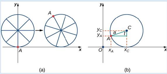
Figure 7.13 (a) The ant clings to the edge of the bicycle tire as the tire rolls along the ground. (b) Using geometry to determine the position of the ant after the tire has rotated through an angle of t.
Note that these are the same parametric representations we had before, but we have now assigned a physical meaning to the parametric variable t.
After a while the ant is getting dizzy from going round and round on the edge of the tire. So he climbs up one of the spokes toward the center of the wheel. By climbing toward the center of the wheel, the ant has changed his path of motion. The new path has less up—and-down motion and is called a curtate cycloid (Figure 7.14). As shown in the figure, we let b denote the distance along the spoke from the center of the wheel to the ant. As before, we let t represent the angle the tire has rotated through. Additionally, we let
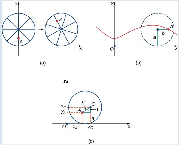
Figure 7.14 (a) The ant climbs up one of the spokes toward the center of the wheel. (b) The ant’s path of motion after he climbs closer to the center of the wheel. This is called a curtate cycloid. (c) The new setup, now that the ant has moved closer to the center of the wheel.
3. On the basis of your answers to parts 1 and 2, what are the parametric equations representing the curtate cycloid?
Once the ant’s head clears, he realizes that the bicyclist has made a turn, and is now traveling away from his home. So he drops off the bicycle tire and looks around. Fortunately, there is a set of train tracks nearby, headed back in the right direction. So the ant heads over to the train tracks to wait. After a while, a train goes by, heading in the right direction, and he manages to jump up and just catch the edge of the train wheel (without getting squished!)
The ant is still worried about getting dizzy, but the train wheel is slippery and has no spokes to climb, so he decides to just hang on to the edge of the wheel and hope for the best. Now, train wheels have a ?ange to keep the wheel running on the tracks. So, in this case, since the ant is hanging on to the very edge of the ?ange, the distance from the center of the wheel to the ant is actually greater than the radius of the wheel (Figure 7.15). The setup here is essentially the same as when the ant climbed up the spoke on the bicycle wheel. We let b denote the distance from the center of the wheel to the ant, and we let t represent the angle the tire has rotated through. Additionally, we let
When the distance from the center of the wheel to the ant is greater than the radius of the wheel, his path of motion is called a prolate cycloid. A graph of a prolate cycloid is shown in the ?gure.
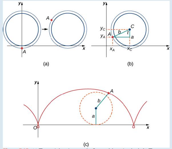
Figure 7.15 (a) The ant is hanging onto-the ?ange of the train wheel. (b) The new setup, now that the ant has jumped onto the train wheel. (c) The ant travels along a prolate cycloid.
Want to see the full answer?
Check out a sample textbook solution
Chapter 7 Solutions
Calculus Volume 2
Additional Math Textbook Solutions
Elementary Statistics (13th Edition)
University Calculus: Early Transcendentals (4th Edition)
A Problem Solving Approach To Mathematics For Elementary School Teachers (13th Edition)
A First Course in Probability (10th Edition)
Calculus: Early Transcendentals (2nd Edition)


- The accompanying data shows the fossil fuels production, fossil fuels consumption, and total energy consumption in quadrillions of BTUs of a certain region for the years 1986 to 2015. Complete parts a and b. Year Fossil Fuels Production Fossil Fuels Consumption Total Energy Consumption1949 28.748 29.002 31.9821950 32.563 31.632 34.6161951 35.792 34.008 36.9741952 34.977 33.800 36.7481953 35.349 34.826 37.6641954 33.764 33.877 36.6391955 37.364 37.410 40.2081956 39.771 38.888 41.7541957 40.133 38.926 41.7871958 37.216 38.717 41.6451959 39.045 40.550 43.4661960 39.869 42.137 45.0861961 40.307 42.758 45.7381962 41.732 44.681 47.8261963 44.037 46.509 49.6441964 45.789 48.543 51.8151965 47.235 50.577 54.0151966 50.035 53.514 57.0141967 52.597 55.127 58.9051968 54.306 58.502 62.4151969 56.286…arrow_forwardCan you check If my short explantions make sense because I want to make sure that I describe this part accuratelyarrow_forwardWe are going to build a snake bot using 6 different segments. How many different snake bots can we make? Show Calculatorarrow_forward
- Bruce and Krista are going to buy a new furniture set for their living room. They want to buy a couch, a coffee table, and a recliner. They have narrowed it down so that they are choosing between \[4\] couches, \[5\] coffee tables, and \[9\] recliners. How many different furniture combinations are possible?arrow_forwardThe accompanying data shows the fossil fuels production, fossil fuels consumption, and total energy consumption in quadrillions of BTUs of a certain region for the years 1986 to 2015. Complete parts a and b. Year Fossil Fuels Production Fossil Fuels Consumption Total Energy Consumption1949 28.748 29.002 31.9821950 32.563 31.632 34.6161951 35.792 34.008 36.9741952 34.977 33.800 36.7481953 35.349 34.826 37.6641954 33.764 33.877 36.6391955 37.364 37.410 40.2081956 39.771 38.888 41.7541957 40.133 38.926 41.7871958 37.216 38.717 41.6451959 39.045 40.550 43.4661960 39.869 42.137 45.0861961 40.307 42.758 45.7381962 41.732 44.681 47.8261963 44.037 46.509 49.6441964 45.789 48.543 51.8151965 47.235 50.577 54.0151966 50.035 53.514 57.0141967 52.597 55.127 58.9051968 54.306 58.502 62.4151969 56.286…arrow_forwardThe accompanying data shows the fossil fuels production, fossil fuels consumption, and total energy consumption in quadrillions of BTUs of a certain region for the years 1986 to 2015. Complete parts a and b. Develop line charts for each variable and identify the characteristics of the time series (that is, random, stationary, trend, seasonal, or cyclical). What is the line chart for the variable Fossil Fuels Production?arrow_forward
- The accompanying data shows the fossil fuels production, fossil fuels consumption, and total energy consumption in quadrillions of BTUs of a certain region for the years 1986 to 2015. Complete parts a and b. Year Fossil Fuels Production Fossil Fuels Consumption Total Energy Consumption1949 28.748 29.002 31.9821950 32.563 31.632 34.6161951 35.792 34.008 36.9741952 34.977 33.800 36.7481953 35.349 34.826 37.6641954 33.764 33.877 36.6391955 37.364 37.410 40.2081956 39.771 38.888 41.7541957 40.133 38.926 41.7871958 37.216 38.717 41.6451959 39.045 40.550 43.4661960 39.869 42.137 45.0861961 40.307 42.758 45.7381962 41.732 44.681 47.8261963 44.037 46.509 49.6441964 45.789 48.543 51.8151965 47.235 50.577 54.0151966 50.035 53.514 57.0141967 52.597 55.127 58.9051968 54.306 58.502 62.4151969 56.286…arrow_forwardFor each of the time series, construct a line chart of the data and identify the characteristics of the time series (that is, random, stationary, trend, seasonal, or cyclical). Month PercentApr 1972 4.97May 1972 5.00Jun 1972 5.04Jul 1972 5.25Aug 1972 5.27Sep 1972 5.50Oct 1972 5.73Nov 1972 5.75Dec 1972 5.79Jan 1973 6.00Feb 1973 6.02Mar 1973 6.30Apr 1973 6.61May 1973 7.01Jun 1973 7.49Jul 1973 8.30Aug 1973 9.23Sep 1973 9.86Oct 1973 9.94Nov 1973 9.75Dec 1973 9.75Jan 1974 9.73Feb 1974 9.21Mar 1974 8.85Apr 1974 10.02May 1974 11.25Jun 1974 11.54Jul 1974 11.97Aug 1974 12.00Sep 1974 12.00Oct 1974 11.68Nov 1974 10.83Dec 1974 10.50Jan 1975 10.05Feb 1975 8.96Mar 1975 7.93Apr 1975 7.50May 1975 7.40Jun 1975 7.07Jul 1975 7.15Aug 1975 7.66Sep 1975 7.88Oct 1975 7.96Nov 1975 7.53Dec 1975 7.26Jan 1976 7.00Feb 1976 6.75Mar 1976 6.75Apr 1976 6.75May 1976…arrow_forwardUsing FDF, BDF, and CDF, find the first derivative; 1. The distance x of a runner from a fixed point is measured (in meters) at an interval of half a second. The data obtained is: t 0 x 0 0.5 3.65 1.0 1.5 2.0 6.80 9.90 12.15 Use CDF to approximate the runner's velocity at times t = 0.5s and t = 1.5s 2. Using FDF, BDF, and CDF, find the first derivative of f(x)=x Inx for an input of 2 assuming a step size of 1. Calculate using Analytical Solution and Absolute Relative Error: = True Value - Approximate Value| x100 True Value 3. Given the data below where f(x) sin (3x), estimate f(1.5) using Langrage Interpolation. x 1 1.3 1.6 1.9 2.2 f(x) 0.14 -0.69 -0.99 -0.55 0.31 4. The vertical distance covered by a rocket from t=8 to t=30 seconds is given by: 30 x = Loo (2000ln 140000 140000 - 2100 9.8t) dt Using the Trapezoidal Rule, n=2, find the distance covered. 5. Use Simpson's 1/3 and 3/8 Rule to approximate for sin x dx. Compare the results for n=4 and n=8arrow_forward
 Algebra and Trigonometry (MindTap Course List)AlgebraISBN:9781305071742Author:James Stewart, Lothar Redlin, Saleem WatsonPublisher:Cengage Learning
 Trigonometry (MindTap Course List)TrigonometryISBN:9781337278461Author:Ron LarsonPublisher:Cengage Learning
 Algebra & Trigonometry with Analytic GeometryAlgebraISBN:9781133382119Author:SwokowskiPublisher:Cengage
 Trigonometry (MindTap Course List)TrigonometryISBN:9781305652224Author:Charles P. McKeague, Mark D. TurnerPublisher:Cengage Learning