
Concept explainers
Videos
Microwave ovens only last so long. The life-time of a microwave oven follows a uniform distribution between 8 and 14 years.
- (a) Draw this uniform distribution. What are the height and base values?
- (b) Show the total area under the curve is 1.00.
- (c) Calculate the mean and the standard deviation of this distribution.
- (d) What is the
probability a particular microwave oven lasts between 10 and 14 years? - (e) What is the probability a microwave oven will last less than 9 years?
a.
Draw the uniform distribution graphically.
Find the height and base values of distribution.
Answer to Problem 1SR
The height and base values of the distribution are 0.167 and 6, respectively.
Explanation of Solution
Step-by-step procedure to obtain the uniform distribution using MINITAB software:
- Choose Graph > Probability Distribution Plot.
- From Distribution, choose Uniform.
- Enter Lower endpoint as 8 and Upper endpoint as 14.
- Click Ok.
The output obtained using MINITAB software is represented as follows:
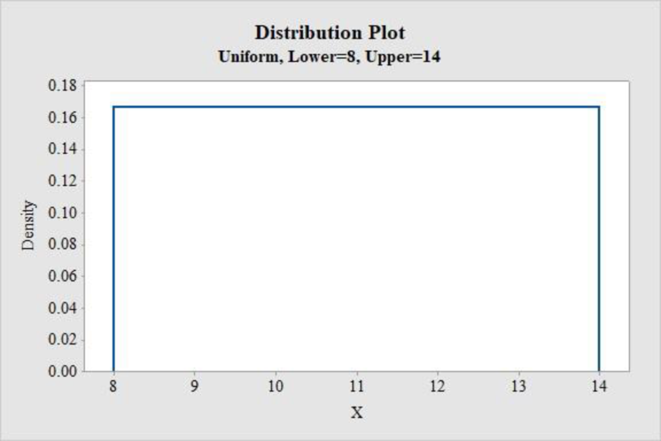
From the above output, the shape of the distribution is rectangle.
The height of the distribution is calculated below:
Therefore, the height of the distribution is 0.167.
The base of the distribution is obtained below:
The base value of the distribution is 6.
b.
Prove that the total area under the curve is 1.00
Explanation of Solution
Let X is the life-time of a microwave oven which follows uniform distribution over the interval from 8 and 14 years.
That is,
The probability density function of a uniform distribution is,
The height and base values of the distribution are 0.167 and 6 respectively.
The area under the curve is obtained below:
Therefore, the total area under the curve is 1.
c.
Compute the mean and standard deviation of the distribution.
Answer to Problem 1SR
The mean of the distribution is 11.
The standard deviation of the distribution is 1.73.
Explanation of Solution
The formula for mean of the distribution is stated below:
The mean life-time of a microwave oven is 11.
The formula for standard deviation of the distribution is computed below:
Therefore, the standard deviation of the distribution is 1.73.
d.
Find the probability that a particular microwave oven lasts between 10 and 14 years.
Answer to Problem 1SR
The probability that a particular microwave oven lasts between 10 and 14 years is 0.668.
Explanation of Solution
The height of the distribution is 0.167 and base of the distribution is 4 ( = 14 – 10).
The probability that a particular microwave oven lasts between 10 and 14 years is,
Therefore, the probability that a particular microwave oven lasts between 10 and 14 years is 0.668.
e.
Find the probability that a microwave oven will last less than 9 years.
Answer to Problem 1SR
The probability that a particular microwave oven will last less than 9 years is 0.167.
Explanation of Solution
The height of the distribution is 0.167 and base of the distribution is 1.
The probability that a particular microwave oven will last less than 9 years is calculated below:
Therefore, the probability that a particular microwave oven will last less than 9 years is 0.167.
Want to see more full solutions like this?
Chapter 7 Solutions
Statistical Techniques in Business and Economics


- Question 2 Parts manufactured by an injection molding process are subjected to a compressive strength test. Twenty samples of five parts each are collected, and the compressive strengths (in psi) are shown in Table 2. Table 2: Strength Data for Question 2 Sample Number x1 x2 23 x4 x5 R 1 83.0 2 88.6 78.3 78.8 3 85.7 75.8 84.3 81.2 78.7 75.7 77.0 71.0 84.2 81.0 79.1 7.3 80.2 17.6 75.2 80.4 10.4 4 80.8 74.4 82.5 74.1 75.7 77.5 8.4 5 83.4 78.4 82.6 78.2 78.9 80.3 5.2 File Preview 6 75.3 79.9 87.3 89.7 81.8 82.8 14.5 7 74.5 78.0 80.8 73.4 79.7 77.3 7.4 8 79.2 84.4 81.5 86.0 74.5 81.1 11.4 9 80.5 86.2 76.2 64.1 80.2 81.4 9.9 10 75.7 75.2 71.1 82.1 74.3 75.7 10.9 11 80.0 81.5 78.4 73.8 78.1 78.4 7.7 12 80.6 81.8 79.3 73.8 81.7 79.4 8.0 13 82.7 81.3 79.1 82.0 79.5 80.9 3.6 14 79.2 74.9 78.6 77.7 75.3 77.1 4.3 15 85.5 82.1 82.8 73.4 71.7 79.1 13.8 16 78.8 79.6 80.2 79.1 80.8 79.7 2.0 17 82.1 78.2 18 84.5 76.9 75.5 83.5 81.2 19 79.0 77.8 20 84.5 73.1 78.2 82.1 79.2 81.1 7.6 81.2 84.4 81.6 80.8…arrow_forwardName: Lab Time: Quiz 7 & 8 (Take Home) - due Wednesday, Feb. 26 Contingency Analysis (Ch. 9) In lab 5, part 3, you will create a mosaic plot and conducted a chi-square contingency test to evaluate whether elderly patients who did not stop walking to talk (vs. those who did stop) were more likely to suffer a fall in the next six months. I have tabulated the data below. Answer the questions below. Please show your calculations on this or a separate sheet. Did not stop walking to talk Stopped walking to talk Totals Suffered a fall Did not suffer a fall Totals 12 11 23 2 35 37 14 14 46 60 Quiz 7: 1. (2 pts) Compute the odds of falling for each group. Compute the odds ratio for those who did not stop walking vs. those who did stop walking. Interpret your result verbally.arrow_forwardSolve please and thank you!arrow_forward
- 7. In a 2011 article, M. Radelet and G. Pierce reported a logistic prediction equation for the death penalty verdicts in North Carolina. Let Y denote whether a subject convicted of murder received the death penalty (1=yes), for the defendant's race h (h1, black; h = 2, white), victim's race i (i = 1, black; i = 2, white), and number of additional factors j (j = 0, 1, 2). For the model logit[P(Y = 1)] = a + ß₁₂ + By + B²², they reported = -5.26, D â BD = 0, BD = 0.17, BY = 0, BY = 0.91, B = 0, B = 2.02, B = 3.98. (a) Estimate the probability of receiving the death penalty for the group most likely to receive it. [4 pts] (b) If, instead, parameters used constraints 3D = BY = 35 = 0, report the esti- mates. [3 pts] h (c) If, instead, parameters used constraints Σ₁ = Σ₁ BY = Σ; B = 0, report the estimates. [3 pts] Hint the probabilities, odds and odds ratios do not change with constraints.arrow_forwardSolve please and thank you!arrow_forwardSolve please and thank you!arrow_forward
- Question 1:We want to evaluate the impact on the monetary economy for a company of two types of strategy (competitive strategy, cooperative strategy) adopted by buyers.Competitive strategy: strategy characterized by firm behavior aimed at obtaining concessions from the buyer.Cooperative strategy: a strategy based on a problem-solving negotiating attitude, with a high level of trust and cooperation.A random sample of 17 buyers took part in a negotiation experiment in which 9 buyers adopted the competitive strategy, and the other 8 the cooperative strategy. The savings obtained for each group of buyers are presented in the pdf that i sent: For this problem, we assume that the samples are random and come from two normal populations of unknown but equal variances.According to the theory, the average saving of buyers adopting a competitive strategy will be lower than that of buyers adopting a cooperative strategy.a) Specify the population identifications and the hypotheses H0 and H1…arrow_forwardYou assume that the annual incomes for certain workers are normal with a mean of $28,500 and a standard deviation of $2,400. What’s the chance that a randomly selected employee makes more than $30,000?What’s the chance that 36 randomly selected employees make more than $30,000, on average?arrow_forwardWhat’s the chance that a fair coin comes up heads more than 60 times when you toss it 100 times?arrow_forward
- Suppose that you have a normal population of quiz scores with mean 40 and standard deviation 10. Select a random sample of 40. What’s the chance that the mean of the quiz scores won’t exceed 45?Select one individual from the population. What’s the chance that his/her quiz score won’t exceed 45?arrow_forwardSuppose that you take a sample of 100 from a population that contains 45 percent Democrats. What sample size condition do you need to check here (if any)?What’s the standard error of ^P?Compare the standard errors of ^p n=100 for ,n=1000 , n=10,000, and comment.arrow_forwardSuppose that a class’s test scores have a mean of 80 and standard deviation of 5. You choose 25 students from the class. What’s the chance that the group’s average test score is more than 82?arrow_forward
 Glencoe Algebra 1, Student Edition, 9780079039897...AlgebraISBN:9780079039897Author:CarterPublisher:McGraw Hill
 Big Ideas Math A Bridge To Success Algebra 1: Stu...AlgebraISBN:9781680331141Author:HOUGHTON MIFFLIN HARCOURTPublisher:Houghton Mifflin Harcourt