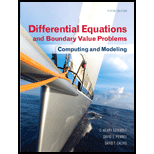
MyLab Math with Pearson eText -- 24-Month Standalone Access Card -- For Differential Equations and Boundary Value Problems: Computing and Modeling Tech Update
5th Edition
ISBN: 9780134872971
Author: Edwards, C., Penney, David, Calvis
Publisher: PEARSON
expand_more
expand_more
format_list_bulleted
Concept explainers
Question
Chapter 6.1, Problem 11P
Program Plan Intro
Write a code to find the equilibrium solution of the give second order differential equation and construct a phase portrait and direction field for first order system.
Expert Solution & Answer
Want to see the full answer?
Check out a sample textbook solution
Students have asked these similar questions
I would like to know the main features about the following 3 key concepts:1. Backup Domain Controller (BDC)2. Access Control List (ACL)3. Dynamic Memory
In cell C21, enter a formula to calculate the number of miles you expect to drive each month. Divide the value of number of miles (cell A5 from the Data sheet) by the average MPG for the vehicle multiplied by the price of a gallon of gas (cell A6 from the Data sheet).
Microsoft Excel
Chapter 6 Solutions
MyLab Math with Pearson eText -- 24-Month Standalone Access Card -- For Differential Equations and Boundary Value Problems: Computing and Modeling Tech Update
Ch. 6.1 - Prob. 1PCh. 6.1 - Prob. 2PCh. 6.1 - Prob. 3PCh. 6.1 - Prob. 4PCh. 6.1 - Prob. 5PCh. 6.1 - Prob. 6PCh. 6.1 - Prob. 7PCh. 6.1 - Prob. 8PCh. 6.1 - Prob. 9PCh. 6.1 - Prob. 10P
Ch. 6.1 - Prob. 11PCh. 6.1 - Prob. 12PCh. 6.1 - Prob. 13PCh. 6.1 - Prob. 14PCh. 6.1 - Prob. 15PCh. 6.1 - Prob. 16PCh. 6.1 - Prob. 17PCh. 6.1 - Prob. 18PCh. 6.1 - Prob. 19PCh. 6.1 - Prob. 20PCh. 6.1 - Prob. 21PCh. 6.1 - Prob. 22PCh. 6.1 - Prob. 23PCh. 6.1 - Prob. 24PCh. 6.1 - Prob. 25PCh. 6.1 - Prob. 26PCh. 6.1 - Prob. 27PCh. 6.1 - Prob. 28PCh. 6.1 - Prob. 29PCh. 6.1 - Prob. 30PCh. 6.2 - Prob. 1PCh. 6.2 - Prob. 2PCh. 6.2 - Prob. 3PCh. 6.2 - Prob. 4PCh. 6.2 - Prob. 5PCh. 6.2 - Prob. 6PCh. 6.2 - Prob. 7PCh. 6.2 - Prob. 8PCh. 6.2 - Prob. 9PCh. 6.2 - Prob. 10PCh. 6.2 - Prob. 11PCh. 6.2 - Prob. 12PCh. 6.2 - Prob. 13PCh. 6.2 - Prob. 14PCh. 6.2 - Prob. 15PCh. 6.2 - Prob. 16PCh. 6.2 - Prob. 17PCh. 6.2 - Prob. 18PCh. 6.2 - Prob. 19PCh. 6.2 - Prob. 20PCh. 6.2 - Prob. 21PCh. 6.2 - Prob. 22PCh. 6.2 - Prob. 23PCh. 6.2 - Prob. 24PCh. 6.2 - Prob. 25PCh. 6.2 - Prob. 26PCh. 6.2 - Prob. 27PCh. 6.2 - Prob. 28PCh. 6.2 - Prob. 29PCh. 6.2 - Prob. 30PCh. 6.2 - Prob. 31PCh. 6.2 - Prob. 32PCh. 6.2 - Prob. 33PCh. 6.2 - Prob. 34PCh. 6.2 - Prob. 35PCh. 6.2 - Prob. 36PCh. 6.2 - Prob. 37PCh. 6.2 - Prob. 38PCh. 6.3 - Prob. 1PCh. 6.3 - Prob. 2PCh. 6.3 - Prob. 3PCh. 6.3 - Prob. 4PCh. 6.3 - Prob. 5PCh. 6.3 - Prob. 6PCh. 6.3 - Prob. 7PCh. 6.3 - Problems 8 through 10 deal with the competition...Ch. 6.3 - Problems 8 through 10 deal with the competition...Ch. 6.3 - Problems 8 through 10 deal with the competition...Ch. 6.3 - Prob. 11PCh. 6.3 - Prob. 12PCh. 6.3 - Prob. 13PCh. 6.3 - Prob. 14PCh. 6.3 - Prob. 15PCh. 6.3 - Prob. 16PCh. 6.3 - Prob. 17PCh. 6.3 - Prob. 18PCh. 6.3 - Prob. 19PCh. 6.3 - Prob. 20PCh. 6.3 - Prob. 21PCh. 6.3 - Prob. 22PCh. 6.3 - Prob. 23PCh. 6.3 - Prob. 24PCh. 6.3 - Prob. 25PCh. 6.3 - Prob. 26PCh. 6.3 - Prob. 27PCh. 6.3 - Prob. 28PCh. 6.3 - Prob. 29PCh. 6.3 - Prob. 30PCh. 6.3 - Prob. 31PCh. 6.3 - Prob. 32PCh. 6.3 - Prob. 33PCh. 6.3 - Prob. 34PCh. 6.4 - Prob. 1PCh. 6.4 - Prob. 2PCh. 6.4 - Prob. 3PCh. 6.4 - Prob. 4PCh. 6.4 - Prob. 5PCh. 6.4 - Prob. 6PCh. 6.4 - Prob. 7PCh. 6.4 - Prob. 8PCh. 6.4 - Prob. 9PCh. 6.4 - Prob. 10PCh. 6.4 - Prob. 11PCh. 6.4 - Prob. 12PCh. 6.4 - Prob. 13PCh. 6.4 - Prob. 14PCh. 6.4 - Prob. 15PCh. 6.4 - Prob. 16PCh. 6.4 - Prob. 17PCh. 6.4 - Prob. 18PCh. 6.4 - Prob. 19PCh. 6.4 - Prob. 20PCh. 6.4 - Prob. 21PCh. 6.4 - Prob. 22PCh. 6.4 - Prob. 23PCh. 6.4 - Prob. 24PCh. 6.4 - Prob. 25PCh. 6.4 - Prob. 26P
Knowledge Booster
Learn more about
Need a deep-dive on the concept behind this application? Look no further. Learn more about this topic, computer-science and related others by exploring similar questions and additional content below.Similar questions
- In cell C16, enter a formula to calculate the price of the vehicle minus your available cash (from cell A3 in the Data worksheet). Use absolute references where appropriate—you will be copying this formula across the row what fomula would i use and how do i solve itarrow_forwardWhat types of data visualizations or tools based on data visualizations have you used professionally, whether in a current or past position? What types of data did they involve? What, in your experience, is the value these data views or tools added to your performance or productivity?arrow_forwardQuestion: Finding the smallest element and its row index and column index in 2D Array: 1. Write a public Java class min2D. 2. In min2D, write a main method. 3. In the main method, create a 2-D array myArray with 2 rows and 5 columns: {{10, 21, 20, 13, 1}, {2, 6, 7, 8, 14}}. 4. Then, use a nested for loop to find the smallest element and its row index and column index. 5. Print the smallest element and its row index and column index on Java Consolearrow_forward
- (using R)The iris data set in R gives the measurements in centimeters of the variables sepal length and width andpetal length and width, respectively, for 50 flowers from each of 3 species of iris, setosa, versicolor, andvirginica. Use the iris data set and the t.test function, test if the mean of pepal length of iris flowers isgreater than the mean of sepal length.The iris data set in R gives the measurements in centimeters of the variables sepal length and width andpetal length and width, respectively, for 50 flowers from each of 3 species of iris, setosa, versicolor, andvirginica. Use the iris data set and the t.test function, test if the mean of pepal length of iris flowers isgreater than the mean of sepal length.arrow_forwardRecognizing the Use of Steganography in Forensic Evidence (4e)Digital Forensics, Investigation, and Response, Fourth Edition - Lab 02arrow_forwardWrite a Java Program to manage student information of a university. The Javaprogram does the following steps:a) The program must use single-dimensional arrays to store the studentinformation such as Student ID, Name and Major.b) The program asks the user to provide the number of students.c) The program asks the user to enter the Student IDs for the number of studentsand stores them.d) The program asks the user to enter the corresponding names for the numberof students and stores them.e) The program then asks the user to provide the corresponding major for thestudents and stores them.f) The program then should display the following options:1. ID Search2. Major Enrollment3. Exitg) On selecting option 1, the user can search for a student using Student ID. Theprogram asks the user to enter a Student ID. It then should print thecorresponding student’s details such as Name and Major if the user providedStudent ID number is present in the stored data. If the user’s Student IDnumber does not…arrow_forward
- (a) Algebraically determine the output state |q3q2q1q0> (which is a 4-qubitvector in 16-dimensional Hilbert space). Show all steps of your calculations. (b) Run a Qiskit code which implements the circuit and append threemeasurement gates to measure the (partial) output state |q2q1q0> (which is a 3-qubit vector in 8-dimensional Hilbert space). this is for quantum soft dev class, you can use stuff like Deutsch Jozsa if u wantarrow_forwardWrite a C++ program that will count from 1 to 10 by 1. The default output should be 1, 2, 3, 4, 5, 6 , 7, 8, 9, 10 There should be only a newline after the last number. Each number except the last should be followed by a comma and a space. To make your program more functional, you should parse command line arguments and change behavior based on their values. Argument Parameter Action -f, --first yes, an integer Change place you start counting -l, --last yes, an integer Change place you end counting -s, --skip optional, an integer, 1 if not specified Change the amount you add to the counter each iteration -h, --help none Print a help message including these instructions. -j, --joke none Tell a number based joke. So, if your program is called counter counter -f 10 --last 4 --skip 2 should produce 10, 8, 6, 4 Please use the last supplied argument. If your code is called counter, counter -f 4 -f 5 -f 6 should count from 6. You should count from first to last inclusively.…arrow_forwardWrite a program that will count from 1 to 10 by 1. The default output should be 1, 2, 3, 4, 5, 6 , 7, 8, 9, 10 There should be only a newline after the last number. Each number except the last should be followed by a comma and a space. To make your program more functional, you should parse command line arguments and change behavior based on their values. Argument Parameter Action -f, --first yes, an integer Change place you start counting -l, --last yes, an integer Change place you end counting -s, --skip optional, an integer, 1 if not specified Change the amount you add to the counter each iteration -h, --help none Print a help message including these instructions. -j, --joke none Tell a number based joke. So, if your program is called counter counter -f 10 --last 4 --skip 2 should produce 10, 8, 6, 4 Please use the last supplied argument. If your code is called counter, counter -f 4 -f 5 -f 6 should count from 6. You should count from first to last inclusively. You…arrow_forward
arrow_back_ios
SEE MORE QUESTIONS
arrow_forward_ios
Recommended textbooks for you
 Operations Research : Applications and AlgorithmsComputer ScienceISBN:9780534380588Author:Wayne L. WinstonPublisher:Brooks Cole
 C++ for Engineers and ScientistsComputer ScienceISBN:9781133187844Author:Bronson, Gary J.Publisher:Course Technology Ptr

Operations Research : Applications and Algorithms
Computer Science
ISBN:9780534380588
Author:Wayne L. Winston
Publisher:Brooks Cole

C++ for Engineers and Scientists
Computer Science
ISBN:9781133187844
Author:Bronson, Gary J.
Publisher:Course Technology Ptr