
Videos
Since laboratory or field experiments are generally expensive and time consuming,
- a. Use the Osman et al. (2008) method [Eqs. (6.15) through (6.18)].
- b. Use the Gurtug and Sridharan (2004) method [Eqs. (6.13) and (6.14)].
- c. Use the Matteo et al. (2009) method [Eqs. (6.19) and (6.20)].
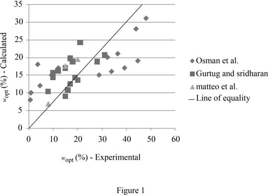
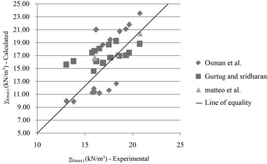
- d. Plot the calculated wopt against the experimental wopt, and the calculated γd(max) with the experimental γd(max). Draw a 45° line of equality on each plot.
- e. Comment on the predictive capabilities of various methods. What can you say about the inherent nature of empirical models?
(a)
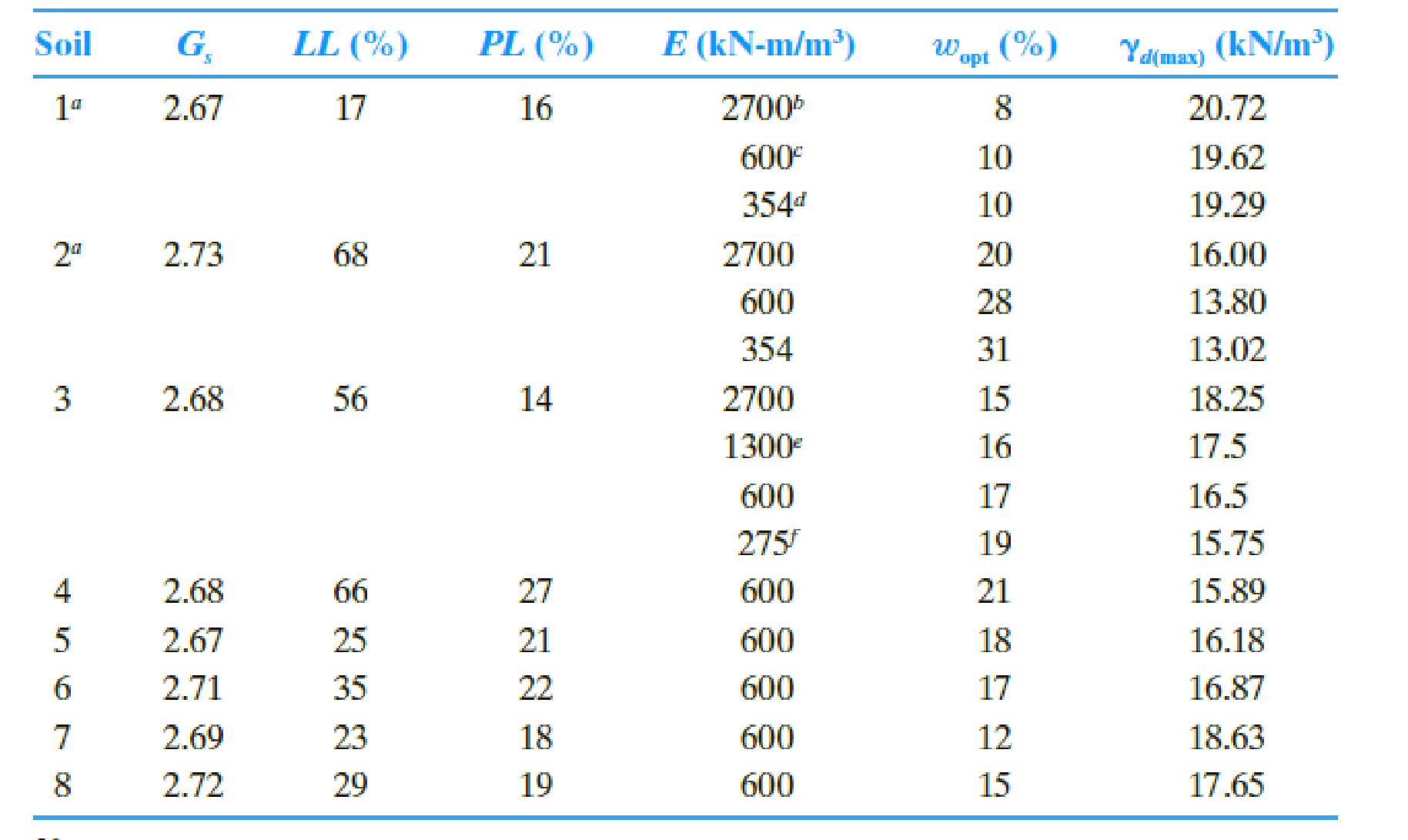
Find the optimum moisture content and maximum dry unit weight using Osman et al. (2008) method.
Explanation of Solution
Calculation:
Determine the plasticity index PI using the relation.
Here, LL is the liquid limit for soil 1 and PL is the plastic limit for soil 1.
Substitute 17 % for LL and 16 % for PL.
Similarly, calculate the PI for remaining soils.
Determine the optimum moisture content for soil 1 using the relation.
Here, E is the compaction energy for soil 1.
Substitute
Similarly, calculate the optimum moisture content for remaining soils.
Determine the value of L using the relation.
Substitute
Determine the value of M using the relation.
Substitute
Determine the maximum dry unit weight of the soil 1 using the relation.
Substitute 23.78 for L, 0.387 for M, and 0.69 % for
Similarly, calculate the maximum dry unit weight for remaining soils.
Summarize the calculated values as in Table 1.
| Soil |
LL (%) |
PL (%) |
PI (%) |
E |
(Exp) |
(Exp) |
| L | M |
|
| 1 | 17 | 16 | 1 | 2,700 | 8 | 20.72 | 0.69 | 23.782 | 0.387 | 23.51 |
| 600 | 10 | 19.62 | 0.93 | 21.984 | 0.277 | 21.73 | ||||
| 354 | 10 | 19.29 | 1.02 | 21.354 | 0.238 | 21.11 | ||||
| 2 | 68 | 21 | 47 | 2,700 | 20 | 16.00 | 32.26 | 23.782 | 0.387 | 11.30 |
| 600 | 28 | 13.80 | 43.92 | 21.984 | 0.277 | 9.82 | ||||
| 354 | 31 | 13.02 | 48.01 | 21.354 | 0.238 | 9.91 | ||||
| 3 | 56 | 14 | 42 | 2,700 | 15 | 18.25 | 28.82 | 23.782 | 0.387 | 12.63 |
| 1,300 | 16 | 17.50 | 33.89 | 22.908 | 0.333 | 11.61 | ||||
| 600 | 17 | 16.50 | 39.24 | 21.984 | 0.277 | 11.12 | ||||
| 275 | 19 | 15.75 | 44.65 | 21.052 | 0.220 | 11.23 | ||||
| 4 | 66 | 27 | 39 | 600 | 21 | 15.89 | 36.45 | 21.984 | 0.277 | 11.89 |
| 5 | 25 | 21 | 4 | 600 | 18 | 16.18 | 3.740 | 21.984 | 0.277 | 20.95 |
| 6 | 35 | 22 | 13 | 600 | 17 | 16.87 | 12.15 | 21.984 | 0.277 | 18.62 |
| 7 | 23 | 18 | 5 | 600 | 12 | 18.63 | 4.67 | 21.984 | 0.277 | 20.69 |
| 8 | 29 | 19 | 10 | 600 | 15 | 17.65 | 9.35 | 21.984 | 0.277 | 19.39 |
(b)
Find the optimum moisture content and maximum dry unit weight using Gurtug and Sridharan (2004) method.
Explanation of Solution
Calculation:
Determine the optimum moisture content for soil 1 using the relation.
Substitute
Determine the maximum dry unit weight of the soil 1 using the relation.
Substitute 10.34 % for
Similarly, calculate the maximum dry unit weight for remaining soils.
Summarize the calculated values as in Table 2.
| Soil |
PL (%) |
E |
(Exp) |
(Exp) |
|
|
| 1 | 16 | 2,700 | 8 | 20.72 | 10.34 | 18.77 |
| 600 | 10 | 19.62 | 14.31 | 17.46 | ||
| 354 | 10 | 19.29 | 15.70 | 17.02 | ||
| 2 | 21 | 2,700 | 20 | 16.00 | 13.57 | 17.69 |
| 600 | 28 | 13.80 | 18.78 | 16.08 | ||
| 354 | 31 | 13.02 | 20.61 | 15.55 | ||
| 3 | 14 | 2,700 | 15 | 18.25 | 9.05 | 19.22 |
| 1,300 | 16 | 17.50 | 10.73 | 18.64 | ||
| 600 | 17 | 16.50 | 12.52 | 18.04 | ||
| 275 | 19 | 15.75 | 14.32 | 17.45 | ||
| 4 | 27 | 600 | 21 | 15.89 | 24.15 | 14.58 |
| 5 | 21 | 600 | 18 | 16.18 | 18.78 | 16.08 |
| 6 | 22 | 600 | 17 | 16.87 | 19.67 | 15.82 |
| 7 | 18 | 600 | 12 | 18.63 | 16.10 | 16.89 |
| 8 | 19 | 600 | 15 | 17.65 | 16.99 | 16.62 |
(c)
Find the optimum moisture content and maximum dry unit weight using Matteo et al. method.
Explanation of Solution
Calculation:
Determine the optimum moisture content for soil 1 using the relation.
Substitute 17 % LL and
Determine the maximum dry unit weight of the soil 1 using the relation.
Substitute 6.94 % for
Similarly, calculate the maximum dry unit weight for remaining soils.
Summarize the calculated values as in Table 3.
| Soil |
Specific gravity |
PI (%) |
(Exp) |
(Exp) |
|
|
| 1 | 2.67 | 1 | 8 | 20.72 | 6.94 | 20.37 |
| 10 | 19.62 | 6.94 | 20.37 | |||
| 10 | 19.29 | 6.94 | 20.37 | |||
| 2 | 2.73 | 47 | 20 | 16.00 | 19.44 | 16.60 |
| 28 | 13.80 | 19.44 | 16.60 | |||
| 31 | 13.02 | 19.44 | 16.60 | |||
| 3 | 2.68 | 42 | 15 | 18.25 | 17.56 | 17.11 |
| 16 | 17.50 | 17.56 | 17.11 | |||
| 17 | 16.50 | 17.56 | 17.11 | |||
| 19 | 15.75 | 17.56 | 17.11 | |||
| 4 | 2.68 | 39 | 21 | 15.89 | 20.31 | 16.25 |
| 5 | 2.67 | 4 | 18 | 16.18 | 9.16 | 19.52 |
| 6 | 2.71 | 13 | 17 | 16.87 | 11.36 | 18.97 |
| 7 | 2.69 | 5 | 12 | 18.63 | 8.41 | 20.25 |
| 8 | 2.72 | 10 | 15 | 17.65 | 9.67 | 19.82 |
(d)
Plot the graph between the calculated
Explanation of Solution
Refer Table 1, 2, and 3.
Draw the graph between the calculated
Draw the graph between calculated
(e)
Comment on the predictive capabilities of various methods and comment about the inherent nature of empirical models.
Explanation of Solution
Prediction of optimum moisture content:
Refer Figure (1), several data points are closely packed around the
Prediction of maximum dry unit weight:
Most data points for all models show good covenant between the calculated and the experimental values.
The empirical models are often limited to the materials, test methods and environmental conditions under which the experiments were conducted and the developed models. For new materials and conditions, the predicted values may not be reliable.
Want to see more full solutions like this?
Chapter 6 Solutions
Bundle: Principles Of Geotechnical Engineering, Loose-leaf Version, 9th + Mindtap Engineering, 1 Term (6 Months) Printed Access Card


- Bars AD and CE (E=105 GPa, a = 20.9×10⁻⁶ °C) support a rigid bar ABC carrying a linearly increasing distributed load as shown. The temperature of Bar CE was then raised by 40°C while the temperature of Bar AD remained unchanged. If Bar AD has a cross-sectional area of 200 mm² while CE has 150 mm², determine the following: the normal force in bar AD, the normal force in bar CE, and the vertical displacement at Point A. D 0.4 m -0.8 m A -0.4 m- B -0.8 m- E 0.8 m C 18 kN/marrow_forwardDraw the updated network. Calculate the new project completion date. Check if there are changes to the completion date and/or to the critical path. Mention the causes for such changes, if any. New network based on the new information received after 15 days (Correct calculations, professionally done). Mention if critical path changes or extended. Write causes for change in critical path or extension in the critical path.arrow_forwardThe single degree of freedom system shown in Figure 3 is at its undeformed position. The SDOF system consists of a rigid beam that is massless. The rigid beam has a pinned (i.e., zero moment) connection to the wall (left end) and it supports a mass m on its right end. The rigid beam is supported by two springs. Both springs have the same stiffness k. The first spring is located at distance L/4 from the left support, where L is the length of the rigid beam. The second spring is located at distance L from the left support.arrow_forward
- For the system shown in Figure 2, u(t) and y(t) denote the absolute displacements of Building A and Building B, respectively. The two buildings are connected using a linear viscous damper with damping coefficient c. Due to construction activity, the floor mass of Building B was estimated that vibrates with harmonic displacement that is described by the following function: y(t) = yocos(2πft). Figure 2: Single-degree-of-freedom system in Problem 2. Please compute the following related to Building A: (a) Derive the equation of motion of the mass m. (20 points) (b) Find the expression of the amplitude of the steady-state displacement of the mass m. (10 pointsarrow_forwardAssume a Space Launch System (Figure 1(a)) that is approximated as a cantilever undamped single degree of freedom (SDOF) system with a mass at its free end (Figure 1(b)). The cantilever is assumed to be massless. Assume a wind load that is approximated with a concentrated harmonic forcing function p(t) = posin(ωt) acting on the mass. The known properties of the SDOF and the applied forcing function are given below. • Mass of SDOF: m =120 kip/g • Acceleration of gravity: g = 386 in/sec2 • Bending sectional stiffness of SDOF: EI = 1015 lbf×in2 • Height of SDOF: h = 2000 inches • Amplitude of forcing function: po = 6 kip • Forcing frequency: f = 8 Hzarrow_forwardA study of the ability of individuals to walk in a straight line reported the accompanying data on cadence (strides per second) for a sample of n = 20 randomly selected healthy men. 0.95 0.85 0.92 0.95 0.93 0.85 1.00 0.92 0.85 0.81 0.78 0.93 0.93 1.05 0.93 1.06 1.08 0.96 0.81 0.96 A normal probability plot gives substantial support to the assumption that the population distribution of cadence is approximately normal. A descriptive summary of the data from Minitab follows. Variable cadence Variable N Mean 20 cadence 0.9260 Min 0.7800 Median 0.9300 Max 1.0800 TrMean 0.9256 Q1 0.8500 StDev 0.0832 Q3 0.9600 SEMean 0.0186 (a) Calculate and interpret a 95% confidence interval for population mean cadence. (Round your answers to two decimal places.) strides per second Interpret this interval. ○ with 95% confidence, the value of the true mean cadence of all such men falls inside the confidence interval. With 95% confidence, the value of the true mean cadence of all such men falls above the…arrow_forward
 Principles of Geotechnical Engineering (MindTap C...Civil EngineeringISBN:9781305970939Author:Braja M. Das, Khaled SobhanPublisher:Cengage Learning
 Fundamentals of Geotechnical Engineering (MindTap...Civil EngineeringISBN:9781305635180Author:Braja M. Das, Nagaratnam SivakuganPublisher:Cengage Learning
 Construction Materials, Methods and Techniques (M...Civil EngineeringISBN:9781305086272Author:William P. Spence, Eva KultermannPublisher:Cengage Learning
 Principles of Foundation Engineering (MindTap Cou...Civil EngineeringISBN:9781337705028Author:Braja M. Das, Nagaratnam SivakuganPublisher:Cengage Learning
 Principles of Foundation Engineering (MindTap Cou...Civil EngineeringISBN:9781305081550Author:Braja M. DasPublisher:Cengage Learning
 Traffic and Highway EngineeringCivil EngineeringISBN:9781305156241Author:Garber, Nicholas J.Publisher:Cengage Learning