Concept explainers
Videos
a.
Find the equation of the least-squares line, if y is expressed in kilograms instead of pounds.
a.
Answer to Problem 28E
The equation of the least-squares line, if y is expressed in kilograms instead of pounds is
Explanation of Solution
Calculation:
The least-squares regression equation relating the shear strength (pounds or lb), y of steel to weld diameter, x is given as
Data transformation:
Software procedure:
Step-by-step procedure to transform the data using the MINITAB software:
- Choose Calc > Calculator.
- Enter the column of y1 under Store result in variable.
- Enter the 0.4536*‘y’ in Expression.
- Click OK in all dialogue boxes.
The transformed data, where each
The least-squares equation can be obtained using software.
Least-squares equation:
Software procedure:
Step-by-step procedure to obtain the least-squares equation using the MINITAB software:
- Choose Stat > Regression > Regression > Fit Regression Model.
- Enter the column of y1 under Responses.
- Enter the column of x under Continuous predictors.
- Choose Results and select Coefficients, Regression Equation.
- Click OK in all dialogue boxes.
Output obtained using MINITAB is given below:
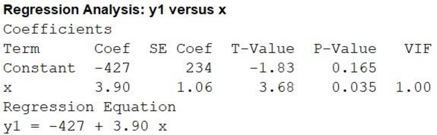
Thus, the equation of the least-squares line, if y is expressed in kilograms instead of pounds is
b.
Find the new slope, intercept, and equation of the least-squares line, if a constant, c is multiplied with every observation on y.
b.
Answer to Problem 28E
The new slope is –936.22 c.
The new intercept is 8.577 c.
The new equation of the least-squares line is
Explanation of Solution
Calculation:
Changing the unit of y from pounds to kilograms causes a change in the scale of y. Now, if the scale of the response variable in a regression, y, is changed by multiplying with a constant c, each least-squares coefficient is also multiplied by c.
Thus, each coefficient in the regression equation, that is, the intercept –936.22 and the slope corresponding to x, 8.577, will be multiplied by c, in order to get the regression equation in this situation. The regression equation is
Thus, the new slope is –936.22 c; the new intercept is 8.577 c; the new equation of the least-squares line is
These can be verified by using the formulae for a and b. The general formulae for a and b, for a simple least-squares regression equation,
Now,
Therefore,
Substitute the values of new a and newb in the general form of the regression equation.
In this problem, a = –936.22 and b = 8.577. As a result, the new slope is –936.22 c; the new intercept is 8.577 c.
Substituting these values in the equation for
Want to see more full solutions like this?
Chapter 5 Solutions
Bundle: Introduction to Statistics and Data Analysis, 5th + WebAssign Printed Access Card: Peck/Olsen/Devore. 5th Edition, Single-Term


- A normal distribution has a mean of 50 and a standard deviation of 4. Solve the following three parts? 1. Compute the probability of a value between 44.0 and 55.0. (The question requires finding probability value between 44 and 55. Solve it in 3 steps. In the first step, use the above formula and x = 44, calculate probability value. In the second step repeat the first step with the only difference that x=55. In the third step, subtract the answer of the first part from the answer of the second part.) 2. Compute the probability of a value greater than 55.0. Use the same formula, x=55 and subtract the answer from 1. 3. Compute the probability of a value between 52.0 and 55.0. (The question requires finding probability value between 52 and 55. Solve it in 3 steps. In the first step, use the above formula and x = 52, calculate probability value. In the second step repeat the first step with the only difference that x=55. In the third step, subtract the answer of the first part from the…arrow_forwardIf a uniform distribution is defined over the interval from 6 to 10, then answer the followings: What is the mean of this uniform distribution? Show that the probability of any value between 6 and 10 is equal to 1.0 Find the probability of a value more than 7. Find the probability of a value between 7 and 9. The closing price of Schnur Sporting Goods Inc. common stock is uniformly distributed between $20 and $30 per share. What is the probability that the stock price will be: More than $27? Less than or equal to $24? The April rainfall in Flagstaff, Arizona, follows a uniform distribution between 0.5 and 3.00 inches. What is the mean amount of rainfall for the month? What is the probability of less than an inch of rain for the month? What is the probability of exactly 1.00 inch of rain? What is the probability of more than 1.50 inches of rain for the month? The best way to solve this problem is begin by a step by step creating a chart. Clearly mark the range, identifying the…arrow_forwardClient 1 Weight before diet (pounds) Weight after diet (pounds) 128 120 2 131 123 3 140 141 4 178 170 5 121 118 6 136 136 7 118 121 8 136 127arrow_forward
- Client 1 Weight before diet (pounds) Weight after diet (pounds) 128 120 2 131 123 3 140 141 4 178 170 5 121 118 6 136 136 7 118 121 8 136 127 a) Determine the mean change in patient weight from before to after the diet (after – before). What is the 95% confidence interval of this mean difference?arrow_forwardIn order to find probability, you can use this formula in Microsoft Excel: The best way to understand and solve these problems is by first drawing a bell curve and marking key points such as x, the mean, and the areas of interest. Once marked on the bell curve, figure out what calculations are needed to find the area of interest. =NORM.DIST(x, Mean, Standard Dev., TRUE). When the question mentions “greater than” you may have to subtract your answer from 1. When the question mentions “between (two values)”, you need to do separate calculation for both values and then subtract their results to get the answer. 1. Compute the probability of a value between 44.0 and 55.0. (The question requires finding probability value between 44 and 55. Solve it in 3 steps. In the first step, use the above formula and x = 44, calculate probability value. In the second step repeat the first step with the only difference that x=55. In the third step, subtract the answer of the first part from the…arrow_forwardIf a uniform distribution is defined over the interval from 6 to 10, then answer the followings: What is the mean of this uniform distribution? Show that the probability of any value between 6 and 10 is equal to 1.0 Find the probability of a value more than 7. Find the probability of a value between 7 and 9. The closing price of Schnur Sporting Goods Inc. common stock is uniformly distributed between $20 and $30 per share. What is the probability that the stock price will be: More than $27? Less than or equal to $24? The April rainfall in Flagstaff, Arizona, follows a uniform distribution between 0.5 and 3.00 inches. What is the mean amount of rainfall for the month? What is the probability of less than an inch of rain for the month? What is the probability of exactly 1.00 inch of rain? What is the probability of more than 1.50 inches of rain for the month? The best way to solve this problem is begin by creating a chart. Clearly mark the range, identifying the lower and upper…arrow_forward
- Problem 1: The mean hourly pay of an American Airlines flight attendant is normally distributed with a mean of 40 per hour and a standard deviation of 3.00 per hour. What is the probability that the hourly pay of a randomly selected flight attendant is: Between the mean and $45 per hour? More than $45 per hour? Less than $32 per hour? Problem 2: The mean of a normal probability distribution is 400 pounds. The standard deviation is 10 pounds. What is the area between 415 pounds and the mean of 400 pounds? What is the area between the mean and 395 pounds? What is the probability of randomly selecting a value less than 395 pounds? Problem 3: In New York State, the mean salary for high school teachers in 2022 was 81,410 with a standard deviation of 9,500. Only Alaska’s mean salary was higher. Assume New York’s state salaries follow a normal distribution. What percent of New York State high school teachers earn between 70,000 and 75,000? What percent of New York State high school…arrow_forwardPls help asaparrow_forwardSolve the following LP problem using the Extreme Point Theorem: Subject to: Maximize Z-6+4y 2+y≤8 2x + y ≤10 2,y20 Solve it using the graphical method. Guidelines for preparation for the teacher's questions: Understand the basics of Linear Programming (LP) 1. Know how to formulate an LP model. 2. Be able to identify decision variables, objective functions, and constraints. Be comfortable with graphical solutions 3. Know how to plot feasible regions and find extreme points. 4. Understand how constraints affect the solution space. Understand the Extreme Point Theorem 5. Know why solutions always occur at extreme points. 6. Be able to explain how optimization changes with different constraints. Think about real-world implications 7. Consider how removing or modifying constraints affects the solution. 8. Be prepared to explain why LP problems are used in business, economics, and operations research.arrow_forward
- ged the variance for group 1) Different groups of male stalk-eyed flies were raised on different diets: a high nutrient corn diet vs. a low nutrient cotton wool diet. Investigators wanted to see if diet quality influenced eye-stalk length. They obtained the following data: d Diet Sample Mean Eye-stalk Length Variance in Eye-stalk d size, n (mm) Length (mm²) Corn (group 1) 21 2.05 0.0558 Cotton (group 2) 24 1.54 0.0812 =205-1.54-05T a) Construct a 95% confidence interval for the difference in mean eye-stalk length between the two diets (e.g., use group 1 - group 2).arrow_forwardAn article in Business Week discussed the large spread between the federal funds rate and the average credit card rate. The table below is a frequency distribution of the credit card rate charged by the top 100 issuers. Credit Card Rates Credit Card Rate Frequency 18% -23% 19 17% -17.9% 16 16% -16.9% 31 15% -15.9% 26 14% -14.9% Copy Data 8 Step 1 of 2: Calculate the average credit card rate charged by the top 100 issuers based on the frequency distribution. Round your answer to two decimal places.arrow_forwardPlease could you check my answersarrow_forward
 Big Ideas Math A Bridge To Success Algebra 1: Stu...AlgebraISBN:9781680331141Author:HOUGHTON MIFFLIN HARCOURTPublisher:Houghton Mifflin Harcourt
 Algebra & Trigonometry with Analytic GeometryAlgebraISBN:9781133382119Author:SwokowskiPublisher:Cengage
 Linear Algebra: A Modern IntroductionAlgebraISBN:9781285463247Author:David PoolePublisher:Cengage Learning