
Videos
a.
Draw a
a.
Answer to Problem 18CRE
The scatterplot for the data is obtained as follows:
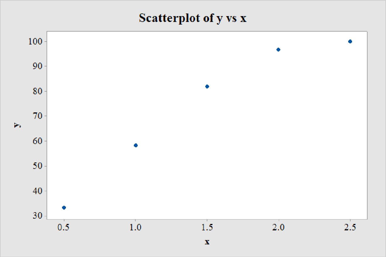
The relationship between the variables is nonlinear.
Explanation of Solution
Calculation:
The data on success (%), y and energy of shock, x is given.
Scatterplot:
Software procedure:
Step-by-step procedure to draw the scatterplot using MINITAB software is given below:
- Choose Graph > Scatterplot.
- Choose Simple, and then click OK.
- Enter the column of y under Y variables.
- Enter the column of x under X variables.
- Click OK.
Thus, the scatterplot is obtained.
A careful observation of the scatterplot reveals that for lower values of x, the points are close to being linear. However, the curvature in the distribution of the points gradually increases with increasing values of x.
Thus, the relationship between the variables is nonlinear.
b.
Fit a least-squares regression line to the data.
Construct a residual plot for the model.
Explain whether the residual plot supports the conclusion in Part a.
b.
Answer to Problem 18CRE
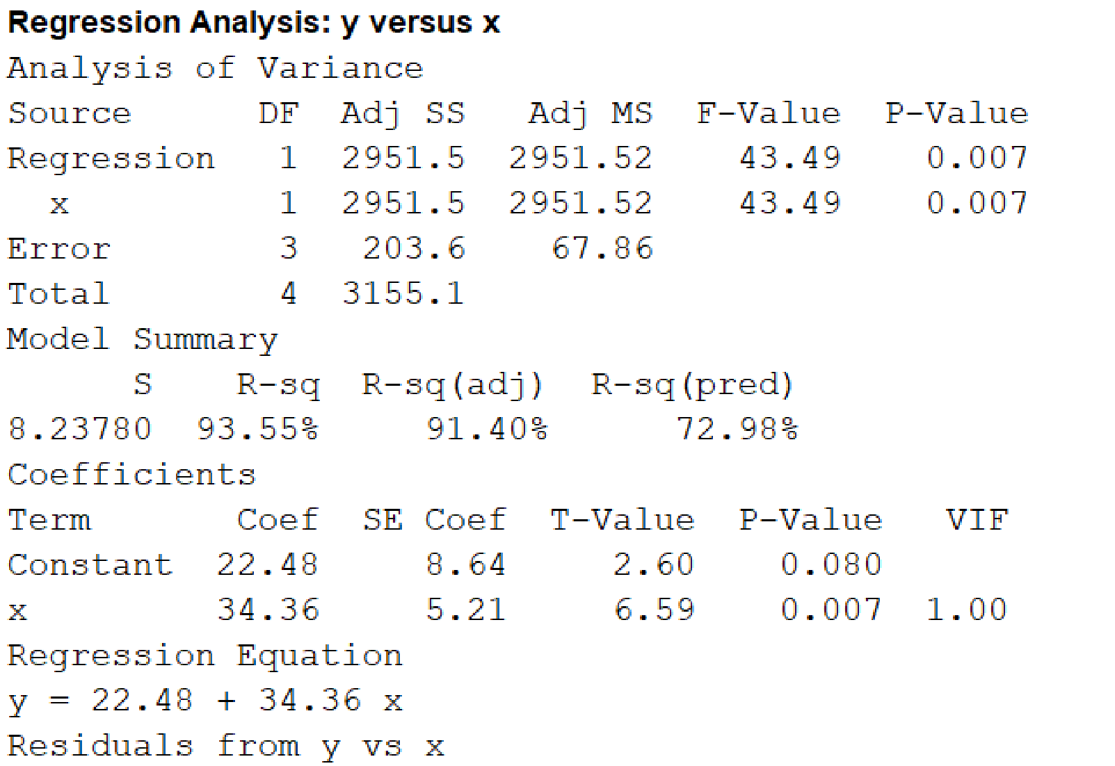
The least-squares regression line for the data is
Explanation of Solution
Calculation:
The least-squares regression line can be obtained using software.
Regression:
Software procedure:
Step by step procedure to get regression equation using MINITAB software is given as,
- Choose Stat > Regression > Regression > Fit Regression Model.
- Under Responses, enter the column of y.
- Under Continuous predictors, enter the columns of x.
- Choose Results and select Analysis of Variance, Model Summary, Coefficients, Regression Equation.
- Choose Graphs, under Residual versus the variables, enter x.
- Click OK on all dialogue boxes.
The outputs using MINITAB software is given as follows:
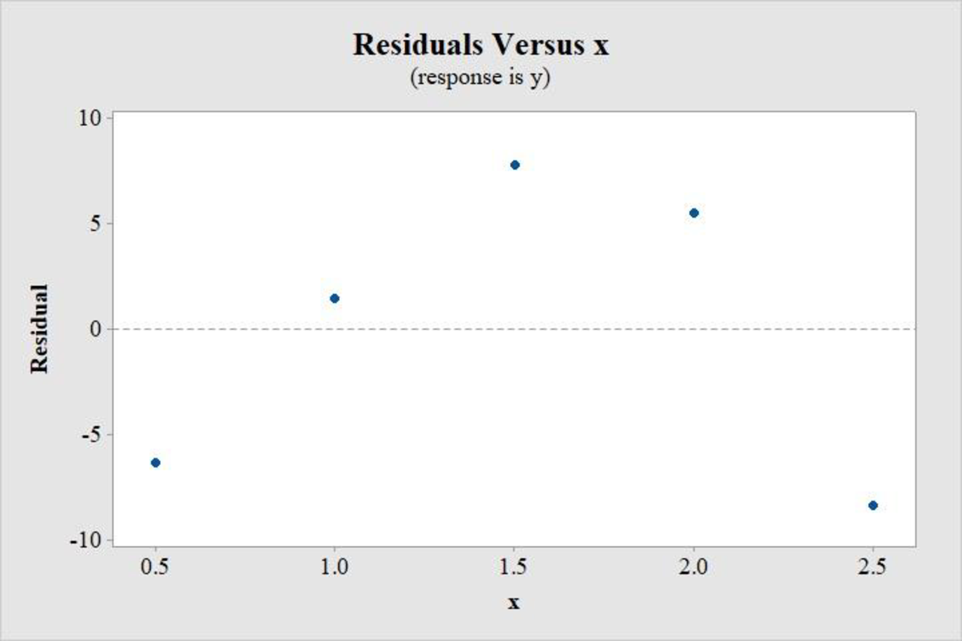
Residual plot:
From the output, the least-squares regression line is:
The ideal residual plot for a linear regression model must not show any pattern and must be randomly distributed. However, this residual plot clearly shows a curved pattern, with an approximate inverted U-shape. This suggests that the data is not linearly distributed.
Thus, the residual plot supports the conclusion in Part a.
c.
Justify whether the transformation
c.
Answer to Problem 18CRE
The transformation
Explanation of Solution
Calculation:
The suitable transformation can be identified by constructing scatterplot between y and
Consider the transformed variable,
Data transformation
Software procedure:
Step-by-step procedure to transform the data using MINITAB software is given below:
- Choose Calc > Calculator.
- Enter the column of sqrt(x) under Store result in variable.
- Enter the formula SQRT(‘x’) under Expression.
- Click OK.
The transformed variable is stored in the column sqrt(x).
Scatterplot:
Software procedure:
Step-by-step procedure to draw the scatterplot using MINITAB software is given below:
- Choose Graph > Scatterplot.
- Choose Simple, and then click OK.
- Enter the column of y under Y variables.
- Enter the column of sqrt(x) under X variables.
- Click OK.
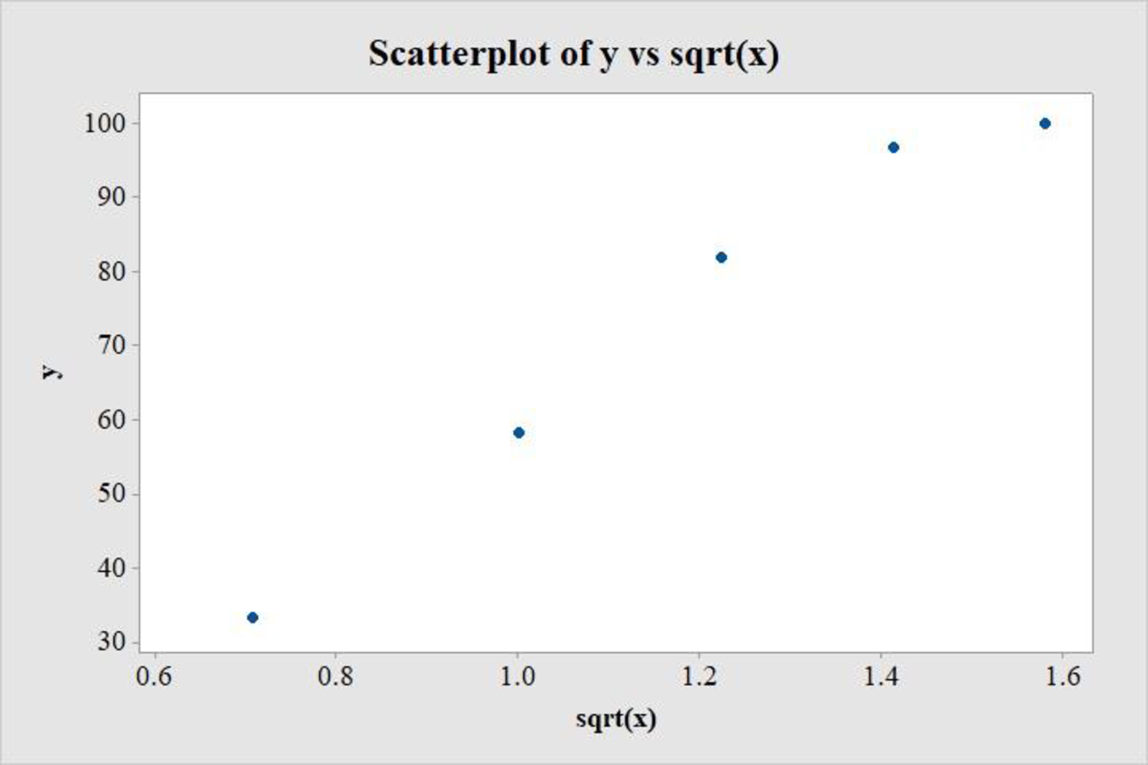
The output obtained using MINITAB is as follows:
Consider the transformed variable,
Data transformation
Software procedure:
Step-by-step procedure to transform the data using MINITAB software is given below:
- Choose Calc > Calculator.
- Enter the column of sqrt(x) under Store result in variable.
- Enter the formula LOGTEN(‘x’) under Expression.
- Click OK.
The transformed variable is stored in the column log(x).
Scatterplot:
Software procedure:
Step-by-step procedure to draw the scatterplot using MINITAB software is given below:
- Choose Graph > Scatterplot.
- Choose Simple, and then click OK.
- Enter the column of y under Y variables.
- Enter the column of log(x) under X variables.
- Click OK.
The output obtained using MINITAB is as follows:
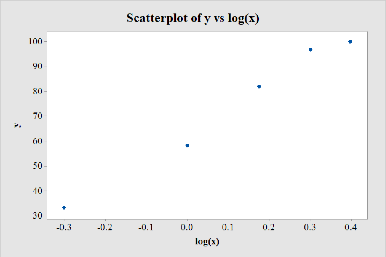
A careful observation of the scatterplot between y and
On the other hand, the scatterplot between y and
Thus, the transformation
d.
Find the least-squares regression line between y and the transformation recommended in the previous part.
d.
Answer to Problem 18CRE
The least-squares regression equation between y and the transformation recommended in the previous part, that is,
Explanation of Solution
Calculation:
The least-squares regression line can be obtained using software.
Regression:
Software procedure:
Step by step procedure to get regression equation using MINITAB software is given as,
- Choose Stat > Regression > Regression > Fit Regression Model.
- Under Responses, enter the column of y.
- Under Continuous predictors, enter the columns of log(x).
- Choose Results and select Analysis of Variance, Model Summary, Coefficients, Regression Equation.
- Click OK on all dialogue boxes.
The outputs using MINITAB software is given as follows:
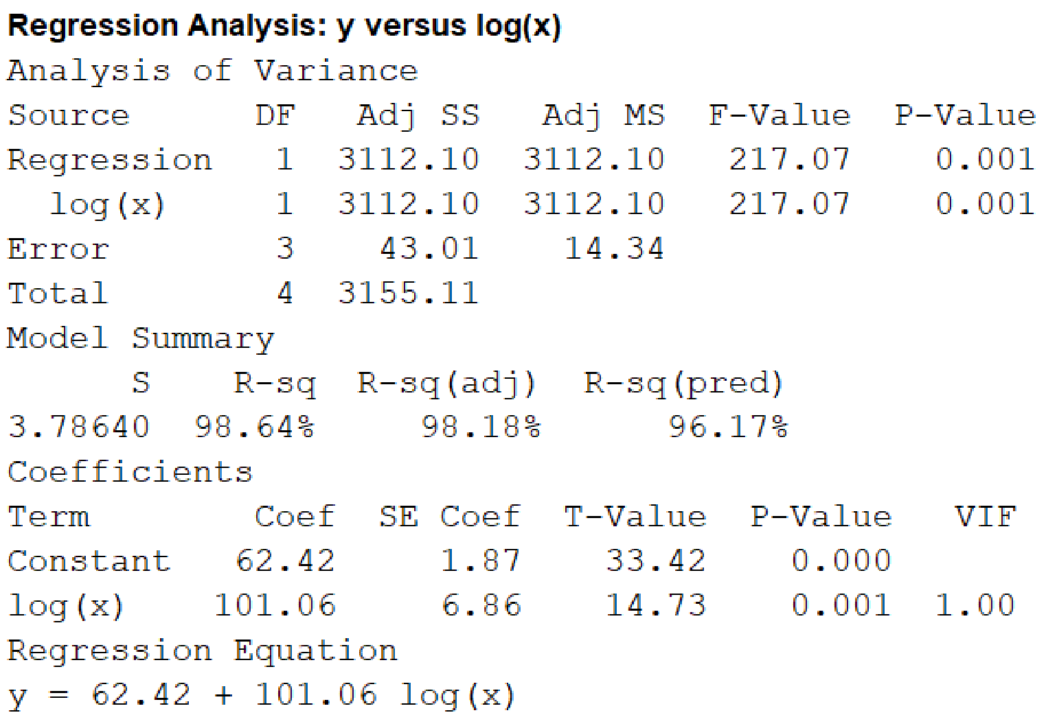
From the output, the least-squares regression equation between y and the transformation recommended in the previous part, that is,
e.
Predict the success for an energy shock 1.75 times the threshold.
Predict the success for an energy shock 0.8 times the threshold.
e.
Answer to Problem 18CRE
The success for an energy shock 1.75 times the threshold is 86.98%.
The success for an energy shock 0.8 times the threshold is 52.63%.
Explanation of Solution
Calculation:
The energy of shock is given as a multiple of the threshold of defibrillation.
For an energy shock 1.75 times the threshold,
Thus, the success for an energy shock 1.75 times the threshold is 86.98%.
For an energy shock 0.8 times the threshold,
Thus, the success for an energy shock 0.8 times the threshold is 52.63%.
Want to see more full solutions like this?
Chapter 5 Solutions
Bundle: Introduction to Statistics and Data Analysis, 5th + WebAssign Printed Access Card: Peck/Olsen/Devore. 5th Edition, Single-Term


- Harvard University California Institute of Technology Massachusetts Institute of Technology Stanford University Princeton University University of Cambridge University of Oxford University of California, Berkeley Imperial College London Yale University University of California, Los Angeles University of Chicago Johns Hopkins University Cornell University ETH Zurich University of Michigan University of Toronto Columbia University University of Pennsylvania Carnegie Mellon University University of Hong Kong University College London University of Washington Duke University Northwestern University University of Tokyo Georgia Institute of Technology Pohang University of Science and Technology University of California, Santa Barbara University of British Columbia University of North Carolina at Chapel Hill University of California, San Diego University of Illinois at Urbana-Champaign National University of Singapore McGill…arrow_forwardName Harvard University California Institute of Technology Massachusetts Institute of Technology Stanford University Princeton University University of Cambridge University of Oxford University of California, Berkeley Imperial College London Yale University University of California, Los Angeles University of Chicago Johns Hopkins University Cornell University ETH Zurich University of Michigan University of Toronto Columbia University University of Pennsylvania Carnegie Mellon University University of Hong Kong University College London University of Washington Duke University Northwestern University University of Tokyo Georgia Institute of Technology Pohang University of Science and Technology University of California, Santa Barbara University of British Columbia University of North Carolina at Chapel Hill University of California, San Diego University of Illinois at Urbana-Champaign National University of Singapore…arrow_forwardA company found that the daily sales revenue of its flagship product follows a normal distribution with a mean of $4500 and a standard deviation of $450. The company defines a "high-sales day" that is, any day with sales exceeding $4800. please provide a step by step on how to get the answers in excel Q: What percentage of days can the company expect to have "high-sales days" or sales greater than $4800? Q: What is the sales revenue threshold for the bottom 10% of days? (please note that 10% refers to the probability/area under bell curve towards the lower tail of bell curve) Provide answers in the yellow cellsarrow_forward
- Find the critical value for a left-tailed test using the F distribution with a 0.025, degrees of freedom in the numerator=12, and degrees of freedom in the denominator = 50. A portion of the table of critical values of the F-distribution is provided. Click the icon to view the partial table of critical values of the F-distribution. What is the critical value? (Round to two decimal places as needed.)arrow_forwardA retail store manager claims that the average daily sales of the store are $1,500. You aim to test whether the actual average daily sales differ significantly from this claimed value. You can provide your answer by inserting a text box and the answer must include: Null hypothesis, Alternative hypothesis, Show answer (output table/summary table), and Conclusion based on the P value. Showing the calculation is a must. If calculation is missing,so please provide a step by step on the answers Numerical answers in the yellow cellsarrow_forwardShow all workarrow_forward
 Glencoe Algebra 1, Student Edition, 9780079039897...AlgebraISBN:9780079039897Author:CarterPublisher:McGraw Hill