Concept explainers
Videos
(a)
Section 1:
To find: The average and standard deviation of
(a)
Section 1:
Answer to Problem 23UYK
Solution: The sampling distribution
Explanation of Solution
Calculation: According to the central limit theorem, when a large sample n is selected from a population, with population average
Standard deviation of the sampling distribution
Section 2:
To find: The average and standard deviation of
Section 2:
Answer to Problem 23UYK
Solution: The sampling distribution
Explanation of Solution
Calculation: According to the central limit theorem, when a large sample n is selected from a population, with population average
Standard deviation of the sampling distribution
Section 3:
To find: The average and standard deviation of
Section 3:
Answer to Problem 23UYK
Solution: The sampling distribution
Explanation of Solution
Calculation: According to the central limit theorem, when a large sample n is selected from a population, with population average
Standard deviation of the sampling distribution
(b)
Section 1:
To find: The population distribution by using the Central Limit Theorem Applet.
(b)
Section 1:
Answer to Problem 23UYK
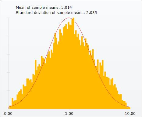
Solution: The distribution of the histogram has an average of 4.963 with standard deviation 2.019.
Explanation of Solution
Calculation: To obtain the population distribution by using the “Central Limit Theorem Applet,” follow the below steps:
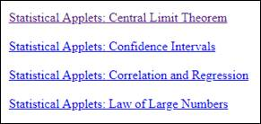
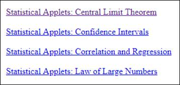
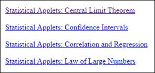
Step 1: Go to “Central Limit Theorem Applet” on the website. The screenshot is shown below:
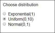
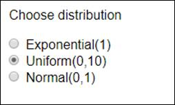
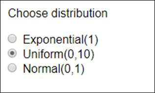
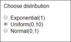
Step 2: Go to Choose distribution and select “Uniform(0,10).” The screenshot is shown below:
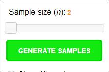
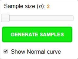
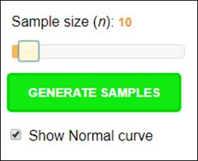
Step 3: Go to
The obtained result is shown below:
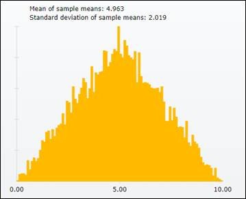
Interpretation: The distribution of the histogram has an average of 4.963 with standard deviation 2.019. All the values are near to the values that is calculated in part (a).
Section 2:
To find: The population distribution by using the Central Limit Theorem Applet.
Section 2:
Answer to Problem 23UYK
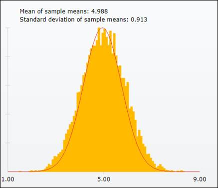
Solution: The distribution of the histogram has an average of 5.016 with standard deviation 0.915.
Explanation of Solution
Calculation: To obtain the population distribution by using the “Central Limit Theorem Applet,” follow the below steps:
Step 1: Go to “Central Limit Theorem Applet” on the website. The screenshot is shown below:
Step 2: Go to Choose distribution and select “Uniform(0,10).” The screenshot is shown below:
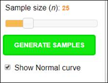
Step 3: Go to Sample size and specify n as “
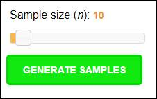
The obtained result is shown below:
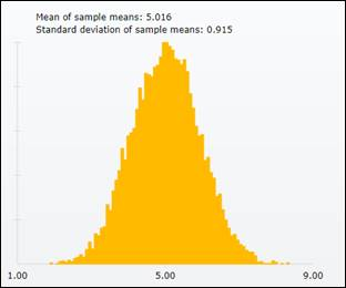
Interpretation: The distribution of the histogram has an average of 5.016 with standard deviation 0.915. All the values are near to the values that are calculated in part (a).
Section 3:
To find: The population distribution by using the Central Limit Theorem Applet.
Section 3:
Answer to Problem 23UYK
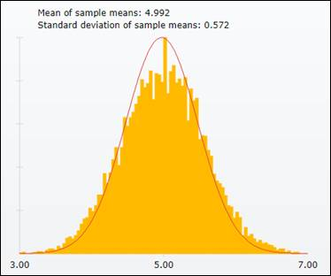
Solution: The distribution of the histogram has an average of 5.005 with standard deviation 0.575.
Explanation of Solution
Calculation: To obtain the population distribution by using the “Central Limit Theorem Applet,” follow the below steps:
Step 1: Go to “Central Limit Theorem Applet” on the website. The screenshot is shown below:
Step 2: Go to Choose distribution and select “Uniform(0,10).” The screenshot is shown below:
Step3: Go to Sample size and specify n as “
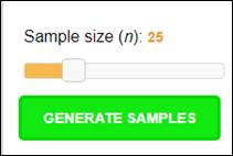
The obtained result is shown below:
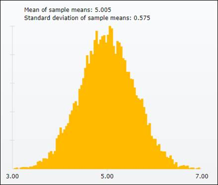
Interpretation: The distribution of the histogram has an average of 5.005 with standard deviation 0.575. All the values are near to the values that are calculated in part (a).
(c)
Section 1:
To find: The shape of the histogram and compare it with the normal plot.
(c)
Section 1:
Answer to Problem 23UYK
Solution: The shape of the distribution has bell-shaped curve. The shape of the histogram is close to the normal curve.
Explanation of Solution
Calculation: To compare the obtained histogram with the normal curve, follow the below steps:
Step 1: Go to “Central Limit Theorem Applet” on the website. The screenshot is shown below:
Step 2: Go to Choose distribution and select “Uniform(0,10).” The screenshot is shown below:
Step 3: Go to Sample size and specify n as “
The obtained result is shown below:
Interpretation: The obtained histogram is
Section 2:
To find: The shape of the histogram and compare it with the normal plot.
Section 2:
Answer to Problem 23UYK
Solution: The shape of the distribution has bell-shaped curve. The shape of the histogram is close to the normal curve.
Explanation of Solution
Calculation: To compare the obtained histogram with the normal curve, follow the steps below:
Step 1: Go to “Central Limit Theorem Applet” on the website. The screenshot is shown below:
Step 2: Go to Choose distribution and select “Uniform(0,10).” The screenshot is shown below:
Step 3: Go to Sample size and specify n as “
The obtained result is shown below:
Interpretation: The obtained histogram is normally distributed with bell-shaped curve. It can be concluded that the shape of the histogram is close to the normal curve.
Section 3:
To find: The shape of the histogram and compare it with the normal plot.
Section 3:
Answer to Problem 23UYK
Solution: The shape of the distribution is bell-shaped curve. The shape of the histogram is close to the normal curve.
Explanation of Solution
Calculation: To compare the obtained histogram with the normal curve, follow the below steps:
Step 1: Go to “Central Limit Theorem Applet” on the website. The screenshot is shown below:
Step 2: Go to Choose distribution and select “Uniform(0,10).” The screenshot is shown below:
Step 3: Go to Sample size and specify n as “
The obtained result is shown below:
Interpretation: The obtained histogram is normally distributed with bell-shaped curve. It can be concluded that the shape of the histogram is close to the normal curve.
(d)
The required sample size.
(d)
Answer to Problem 23UYK
Solution: The sample size should be 25.
Explanation of Solution
Want to see more full solutions like this?
Chapter 5 Solutions
EBK INTRODUCTION TO THE PRACTICE OF STA


- 1) and let Xt is stochastic process with WSS and Rxlt t+t) 1) E (X5) = \ 1 2 Show that E (X5 = X 3 = 2 (= = =) Since X is WSSEL 2 3) find E(X5+ X3)² 4) sind E(X5+X2) J=1 ***arrow_forwardProve that 1) | RxX (T) | << = (R₁ " + R$) 2) find Laplalse trans. of Normal dis: 3) Prove thy t /Rx (z) | < | Rx (0)\ 4) show that evary algebra is algebra or not.arrow_forwardFor each of the time series, construct a line chart of the data and identify the characteristics of the time series (that is, random, stationary, trend, seasonal, or cyclical). Month Number (Thousands)Dec 1991 65.60Jan 1992 71.60Feb 1992 78.80Mar 1992 111.60Apr 1992 107.60May 1992 115.20Jun 1992 117.80Jul 1992 106.20Aug 1992 109.90Sep 1992 106.00Oct 1992 111.80Nov 1992 84.50Dec 1992 78.60Jan 1993 70.50Feb 1993 74.60Mar 1993 95.50Apr 1993 117.80May 1993 120.90Jun 1993 128.50Jul 1993 115.30Aug 1993 121.80Sep 1993 118.50Oct 1993 123.30Nov 1993 102.30Dec 1993 98.70Jan 1994 76.20Feb 1994 83.50Mar 1994 134.30Apr 1994 137.60May 1994 148.80Jun 1994 136.40Jul 1994 127.80Aug 1994 139.80Sep 1994 130.10Oct 1994 130.60Nov 1994 113.40Dec 1994 98.50Jan 1995 84.50Feb 1995 81.60Mar 1995 103.80Apr 1995 116.90May 1995 130.50Jun 1995 123.40Jul 1995 129.10Aug 1995…arrow_forward
- For each of the time series, construct a line chart of the data and identify the characteristics of the time series (that is, random, stationary, trend, seasonal, or cyclical). Year Month Units1 Nov 42,1611 Dec 44,1862 Jan 42,2272 Feb 45,4222 Mar 54,0752 Apr 50,9262 May 53,5722 Jun 54,9202 Jul 54,4492 Aug 56,0792 Sep 52,1772 Oct 50,0872 Nov 48,5132 Dec 49,2783 Jan 48,1343 Feb 54,8873 Mar 61,0643 Apr 53,3503 May 59,4673 Jun 59,3703 Jul 55,0883 Aug 59,3493 Sep 54,4723 Oct 53,164arrow_forwardHigh Cholesterol: A group of eight individuals with high cholesterol levels were given a new drug that was designed to lower cholesterol levels. Cholesterol levels, in milligrams per deciliter, were measured before and after treatment for each individual, with the following results: Individual Before 1 2 3 4 5 6 7 8 237 282 278 297 243 228 298 269 After 200 208 178 212 174 201 189 185 Part: 0/2 Part 1 of 2 (a) Construct a 99.9% confidence interval for the mean reduction in cholesterol level. Let a represent the cholesterol level before treatment minus the cholesterol level after. Use tables to find the critical value and round the answers to at least one decimal place.arrow_forwardI worked out the answers for most of this, and provided the answers in the tables that follow. But for the total cost table, I need help working out the values for 10%, 11%, and 12%. A pharmaceutical company produces the drug NasaMist from four chemicals. Today, the company must produce 1000 pounds of the drug. The three active ingredients in NasaMist are A, B, and C. By weight, at least 8% of NasaMist must consist of A, at least 4% of B, and at least 2% of C. The cost per pound of each chemical and the amount of each active ingredient in one pound of each chemical are given in the data at the bottom. It is necessary that at least 100 pounds of chemical 2 and at least 450 pounds of chemical 3 be used. a. Determine the cheapest way of producing today’s batch of NasaMist. If needed, round your answers to one decimal digit. Production plan Weight (lbs) Chemical 1 257.1 Chemical 2 100 Chemical 3 450 Chemical 4 192.9 b. Use SolverTable to see how much the percentage of…arrow_forward
- At the beginning of year 1, you have $10,000. Investments A and B are available; their cash flows per dollars invested are shown in the table below. Assume that any money not invested in A or B earns interest at an annual rate of 2%. a. What is the maximized amount of cash on hand at the beginning of year 4.$ ___________ A B Time 0 -$1.00 $0.00 Time 1 $0.20 -$1.00 Time 2 $1.50 $0.00 Time 3 $0.00 $1.90arrow_forwardFor each of the time series, construct a line chart of the data and identify the characteristics of the time series (that is, random, stationary, trend, seasonal, or cyclical). Year Month Rate (%)2009 Mar 8.72009 Apr 9.02009 May 9.42009 Jun 9.52009 Jul 9.52009 Aug 9.62009 Sep 9.82009 Oct 10.02009 Nov 9.92009 Dec 9.92010 Jan 9.82010 Feb 9.82010 Mar 9.92010 Apr 9.92010 May 9.62010 Jun 9.42010 Jul 9.52010 Aug 9.52010 Sep 9.52010 Oct 9.52010 Nov 9.82010 Dec 9.32011 Jan 9.12011 Feb 9.02011 Mar 8.92011 Apr 9.02011 May 9.02011 Jun 9.12011 Jul 9.02011 Aug 9.02011 Sep 9.02011 Oct 8.92011 Nov 8.62011 Dec 8.52012 Jan 8.32012 Feb 8.32012 Mar 8.22012 Apr 8.12012 May 8.22012 Jun 8.22012 Jul 8.22012 Aug 8.12012 Sep 7.82012 Oct…arrow_forwardFor each of the time series, construct a line chart of the data and identify the characteristics of the time series (that is, random, stationary, trend, seasonal, or cyclical). Date IBM9/7/2010 $125.959/8/2010 $126.089/9/2010 $126.369/10/2010 $127.999/13/2010 $129.619/14/2010 $128.859/15/2010 $129.439/16/2010 $129.679/17/2010 $130.199/20/2010 $131.79 a. Construct a line chart of the closing stock prices data. Choose the correct chart below.arrow_forward
- For each of the time series, construct a line chart of the data and identify the characteristics of the time series (that is, random, stationary, trend, seasonal, or cyclical) Date IBM9/7/2010 $125.959/8/2010 $126.089/9/2010 $126.369/10/2010 $127.999/13/2010 $129.619/14/2010 $128.859/15/2010 $129.439/16/2010 $129.679/17/2010 $130.199/20/2010 $131.79arrow_forward1. A consumer group claims that the mean annual consumption of cheddar cheese by a person in the United States is at most 10.3 pounds. A random sample of 100 people in the United States has a mean annual cheddar cheese consumption of 9.9 pounds. Assume the population standard deviation is 2.1 pounds. At a = 0.05, can you reject the claim? (Adapted from U.S. Department of Agriculture) State the hypotheses: Calculate the test statistic: Calculate the P-value: Conclusion (reject or fail to reject Ho): 2. The CEO of a manufacturing facility claims that the mean workday of the company's assembly line employees is less than 8.5 hours. A random sample of 25 of the company's assembly line employees has a mean workday of 8.2 hours. Assume the population standard deviation is 0.5 hour and the population is normally distributed. At a = 0.01, test the CEO's claim. State the hypotheses: Calculate the test statistic: Calculate the P-value: Conclusion (reject or fail to reject Ho): Statisticsarrow_forward21. find the mean. and variance of the following: Ⓒ x(t) = Ut +V, and V indepriv. s.t U.VN NL0, 63). X(t) = t² + Ut +V, U and V incepires have N (0,8) Ut ①xt = e UNN (0162) ~ X+ = UCOSTE, UNNL0, 62) SU, Oct ⑤Xt= 7 where U. Vindp.rus +> ½ have NL, 62). ⑥Xn = ΣY, 41, 42, 43, ... Yn vandom sample K=1 Text with mean zen and variance 6arrow_forward
 MATLAB: An Introduction with ApplicationsStatisticsISBN:9781119256830Author:Amos GilatPublisher:John Wiley & Sons Inc
 Probability and Statistics for Engineering and th...StatisticsISBN:9781305251809Author:Jay L. DevorePublisher:Cengage Learning
 Statistics for The Behavioral Sciences (MindTap C...StatisticsISBN:9781305504912Author:Frederick J Gravetter, Larry B. WallnauPublisher:Cengage Learning
 Elementary Statistics: Picturing the World (7th E...StatisticsISBN:9780134683416Author:Ron Larson, Betsy FarberPublisher:PEARSON
 The Basic Practice of StatisticsStatisticsISBN:9781319042578Author:David S. Moore, William I. Notz, Michael A. FlignerPublisher:W. H. Freeman
 Introduction to the Practice of StatisticsStatisticsISBN:9781319013387Author:David S. Moore, George P. McCabe, Bruce A. CraigPublisher:W. H. Freeman