Chapter 5.1, Problem 7UYK

(a)

Section 1:

To determine

To find: The average and standard deviation of $\overline{x}$ for $n=2$.

Answer to Problem 7UYK

Solution: The sampling distribution $\overline{x}$ has an average of 5 with standard deviation 2.04.

Explanation of Solution

Calculation: According to the central limit theorem, when a large sample n is selected from a population, with population average $\mu$ and standard deviation $\sigma$, the sampling distribution $\overline{x}$ will be approximately normal. Mean of the sampling distribution $\overline{x}$ can be calculated as follows:

$\begin{array}{c}{\mu }_{\overline{x}}=\mu \\ =5\end{array}$

Standard deviation of the sampling distribution $\overline{x}$ with $n=2$ can be calculated as follows:

$\begin{array}{c}{\sigma }_{\overline{x}}=\frac{\sigma }{\sqrt{n}}\\ =\frac{2.89}{\sqrt{2}}\\ =2.04\end{array}$

Section 2:

To determine

To find: The average and standard deviation of $\overline{x}$ for $n=10$.

Answer to Problem 7UYK

Solution: The sampling distribution $\overline{x}$ has an average of 5 with standard deviation 0.91.

Explanation of Solution

Calculation: According to the central limit theorem, when a large sample n is selected from a population, with population average $\mu$ and standard deviation $\sigma$, then $\overline{x}$ will be approximately normal. Mean of the sampling distribution $\overline{x}$ can be calculated as follows:

$\begin{array}{c}{\mu }_{\overline{x}}=\mu \\ =5\end{array}$

Standard deviation of the sampling distribution $\overline{x}$ with $n=10$ can be calculated as follows:

$\begin{array}{c}{\sigma }_{\overline{x}}=\frac{\sigma }{\sqrt{n}}\\ =\frac{2.89}{\sqrt{10}}\\ =0.91\end{array}$

Section 3:

To determine

To find: The average and standard deviation of $\overline{x}$ for $n=25$.

Answer to Problem 7UYK

Solution: The sampling distribution $\overline{x}$ has an average of 5 with standard deviation 0.578.

Explanation of Solution

Calculation: According to the central limit theorem, when a large sample n is selected from a population, with population average $\mu$ and standard deviation $\sigma$, then the $\overline{x}$ will be approximately normal. Mean of the sampling distribution $\overline{x}$ can be calculated as follows:

$\begin{array}{c}{\mu }_{\overline{x}}=\mu \\ =5\end{array}$

Standard deviation of the sampling distribution $\overline{x}$ with $n=25$ can be calculated as follows:

$\begin{array}{c}{\sigma }_{\overline{x}}=\frac{\sigma }{\sqrt{n}}\\ =\frac{2.89}{\sqrt{25}}\\ =0.578\end{array}$

(b)

Section 1:

To determine

To find: The population distribution by using the Central Limit Theorem Applet.

Answer to Problem 7UYK

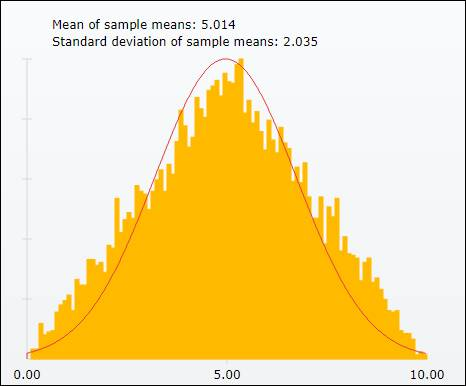
Solution: The distribution of the histogram has an average of 4.963 with standard deviation 2.019.

Explanation of Solution

Calculation: To obtain the population distribution by using the “Central Limit Theorem Applet,” follow the below steps:

Step 1: Go to “Central Limit Theorem Applet” on the website. The screenshot is shown below:

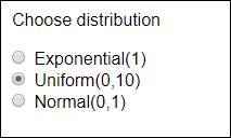
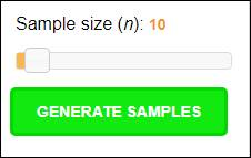
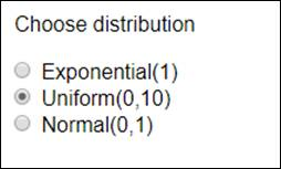
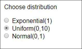
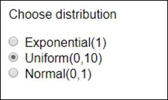
Step 2: Go to Choose distribution and select “Uniform(0,10).” The screenshot is shown below:

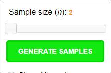
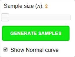
Step 3: Go to Sample size and specify n as “ $n=2$,” and click on “Generate Samples.” The screenshot is shown below:

The obtained result is shown below:

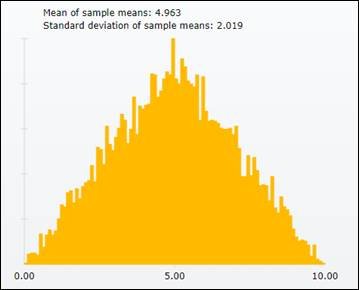
Interpretation: The distribution of the histogram has an average of 4.963 with standard deviation 2.019. All the values are near to the values that is calculated in part (a).

Section 2:

To determine

To find: The population distribution by using the Central Limit Theorem Applet.

Answer to Problem 7UYK

Solution: The distribution of the histogram has an average of 5.016 with standard deviation 0.915.

Explanation of Solution

Calculation: To obtain the population distribution by using the “Central Limit Theorem Applet,” follow the below steps:

Step 1: Go to “Central Limit Theorem Applet” on the website. The screenshot is shown below:

Step 2: Go to Choose distribution and select “Uniform(0,10).” The screenshot is shown below:

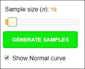
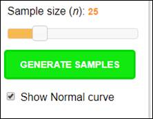
Step 3: Go to Sample size and specify n as “ $n=10$,” and click on “Generate Samples.” The screenshot is shown below:

The obtained result is shown below:

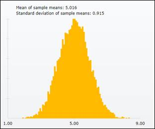
Interpretation: The distribution of the histogram has an average of 5.016 with standard deviation 0.915. All the values are near to the values that are calculated in part (a).

Section 3:

To determine

To find: The population distribution by using the Central Limit Theorem Applet.

Answer to Problem 7UYK

Solution: The distribution of the histogram has an average of 5.005 with standard deviation 0.575.

Explanation of Solution

Calculation: To obtain the population distribution by using the “Central Limit Theorem Applet,” follow the below steps:

Step 1: Go to “Central Limit Theorem Applet” on the website. The screenshot is shown below:

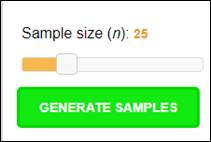
Step 2: Go to Choose distribution and select “Uniform(0,10).” The screenshot is shown below:

Step3: Go to Sample size and specify n as “ $n=25$,” and click on “Generate Samples.” The screenshot is shown below:

The obtained result is shown below:

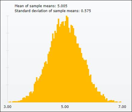
Interpretation: The distribution of the histogram has an average of 5.005 with standard deviation 0.575. All the values are near to the values that are calculated in part (a).

(c)

Section 1:

To determine

To find: The shape of the histogram and compare it with the normal plot.

Answer to Problem 7UYK

Solution: The shape of the distribution has bell-shaped curve. The shape of the histogram is close to the normal curve.

Explanation of Solution

Calculation: To compare the obtained histogram with the normal curve, follow the below steps:

Step 1: Go to “Central Limit Theorem Applet” on the website. The screenshot is shown below:

Step 2: Go to Choose distribution and select “Uniform(0,10).” The screenshot is shown below:

Step 3: Go to Sample size and specify n as “ $n=2$,” and click on “Generate Samples.” Select the column “Show Normal curve.” The screenshot is shown below:

The obtained result is shown below:

Interpretation: The obtained histogram is normally distributed with bell-shaped curve. It can be concluded that the shape of the histogram is close to the normal curve.

Section 2:

To determine

To find: The shape of the histogram and compare it with the normal plot.

Answer to Problem 7UYK

Solution: The shape of the distribution has bell-shaped curve. The shape of the histogram is close to the normal curve.

Explanation of Solution

Calculation: To compare the obtained histogram with the normal curve, follow the steps below:

Step 1: Go to “Central Limit Theorem Applet” on the website. The screenshot is shown below:

Step 2: Go to Choose distribution and select “Uniform(0,10).” The screenshot is shown below:

Step 3: Go to Sample size and specify n as “ $n=10$,” and click on “Generate Samples.” Select the column “Show Normal curve.” The screenshot is shown below:

The obtained result is shown below:

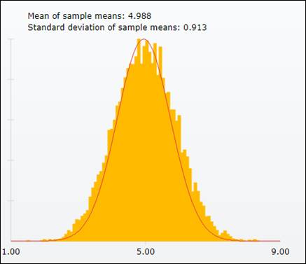
Interpretation: The obtained histogram is normally distributed with bell-shaped curve. It can be concluded that the shape of the histogram is close to the normal curve.

Section 3:

To determine

To find: The shape of the histogram and compare it with the normal plot.

Answer to Problem 7UYK

Solution: The shape of the distribution is bell-shaped curve. The shape of the histogram is close to the normal curve.

Explanation of Solution

Calculation: To compare the obtained histogram with the normal curve, follow the below steps:

Step 1: Go to “Central Limit Theorem Applet” on the website. The screenshot is shown below:

Step 2: Go to Choose distribution and select “Uniform(0,10).” The screenshot is shown below:

Step 3: Go to Sample size and specify n as “ $n=25$,” and click on “Generate Samples.” Select the column “Show Normal curve.” The screenshot is shown below:

The obtained result is shown below:

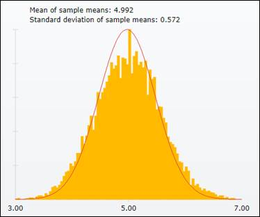
Interpretation: The obtained histogram is normally distributed with bell-shaped curve. It can be concluded that the shape of the histogram is close to the normal curve.

(d)

To determine

The required sample size.

Answer to Problem 7UYK

Solution: The sample size should be 25.

Explanation of Solution

It can be seen in the above parts that curves are approximately normally distributed. According to the central limit theorem, as sample size increases, the shape of the curve moves near to the normal curve. So, the larger sample size is suitable for the use of central limit theorem. Hence, for the provided distribution sample size suitable for the use of central limit theorem is 25.