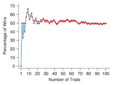
Law of Large Numbers: Gambling Betty and Jane are gambling. They are cutting cards (picking a random place in the deck to see a card). Whoever has the higher card wins the bet. If the cards have the same value (for example, they are both eights), they try again. Betty and Jane do this a 100 times. Tom and Bill are doing the same thing but are betting only 10 times. Is Bill or Betty more likely to end having very close to 50% wins? Explain. You may refer to the graph to help you decide. It is one simulation based on 100 trials.
Law of Large Numbers: Gambling Betty and Jane are gambling. They are cutting cards (picking a random place in the deck to see a card). Whoever has the higher card wins the bet. If the cards have the same value (for example, they are both eights), they try again. Betty and Jane do this a 100 times. Tom and Bill are doing the same thing but are betting only 10 times. Is Bill or Betty more likely to end having very close to 50% wins? Explain. You may refer to the graph to help you decide. It is one simulation based on 100 trials.
Solution Summary: The author explains that Betty is more likely to end up having very close to 50% wins. The graph shows the percentage of wins for different number of trials.
Law of Large Numbers: Gambling Betty and Jane are gambling. They are cutting cards (picking a random place in the deck to see a card). Whoever has the higher card wins the bet. If the cards have the same value (for example, they are both eights), they try again. Betty and Jane do this a 100 times. Tom and Bill are doing the same thing but are betting only 10 times. Is Bill or Betty more likely to end having very close to 50% wins? Explain. You may refer to the graph to help you decide. It is one simulation based on 100 trials.
NC Current Students - North Ce X | NC Canvas Login Links - North ( X
Final Exam Comprehensive x Cengage Learning
x
WASTAT - Final Exam - STAT
→
C
webassign.net/web/Student/Assignment-Responses/submit?dep=36055360&tags=autosave#question3659890_9
Part (b)
Draw a scatter plot of the ordered pairs.
N
Life
Expectancy
Life
Expectancy
80
70
600
50
40
30
20
10
Year of
1950
1970 1990
2010 Birth
O
Life
Expectancy
Part (c)
800
70
60
50
40
30
20
10
1950
1970 1990
W
ALT
林
$
#
4
R
J7
Year of
2010 Birth
F6
4+
80
70
60
50
40
30
20
10
Year of
1950 1970 1990
2010 Birth
Life
Expectancy
Ox
800
70
60
50
40
30
20
10
Year of
1950 1970 1990 2010 Birth
hp
P.B.
KA
&
7
80
% 5
H
A
B
F10
711
N
M
K
744
PRT SC
ALT
CTRL
Chapter 5 Solutions
Pearson eText Introductory Statistics: Exploring the World Through Data -- Instant Access (Pearson+)
Calculus for Business, Economics, Life Sciences, and Social Sciences (14th Edition)
Knowledge Booster
Learn more about
Need a deep-dive on the concept behind this application? Look no further. Learn more about this topic, statistics and related others by exploring similar questions and additional content below.
Discrete Distributions: Binomial, Poisson and Hypergeometric | Statistics for Data Science; Author: Dr. Bharatendra Rai;https://www.youtube.com/watch?v=lHhyy4JMigg;License: Standard Youtube License


 College Algebra (MindTap Course List)AlgebraISBN:9781305652231Author:R. David Gustafson, Jeff HughesPublisher:Cengage Learning
 Holt Mcdougal Larson Pre-algebra: Student Edition...AlgebraISBN:9780547587776Author:HOLT MCDOUGALPublisher:HOLT MCDOUGAL
 Glencoe Algebra 1, Student Edition, 9780079039897...AlgebraISBN:9780079039897Author:CarterPublisher:McGraw Hill
 Algebra & Trigonometry with Analytic GeometryAlgebraISBN:9781133382119Author:SwokowskiPublisher:Cengage