
Concept explainers
Videos
a.
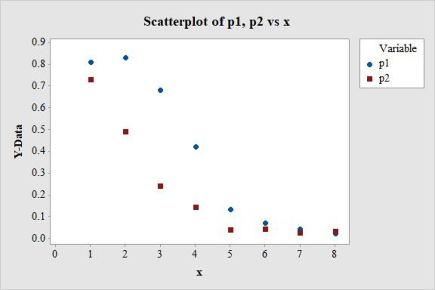
Draw the plots of the proportion of bird eggs hatching for the lowlands and mid-elevation areas versus exposure time.
Identify whether the shapes of the plots are as expected in case of “logistic” plots.
a.
Answer to Problem 71E
The plot of the proportion of bird eggs hatching for the lowlands and mid-elevation areas versus exposure time is as follows:
Explanation of Solution
Calculation:
The given data relates the proportion of bird eggs hatching for the lowlands, mid-elevation areas and cloud-forests with exposure time (days).
Denote the proportion of hatching for lowlands as
Software procedure:
Step-by-step procedure to draw the scatterplots using MINITAB software is given below:
- Choose Graph > Scatterplot.
- Choose Simple, and then click OK.
- Enter the column of p1 in the first cell under Y variables.
- Enter the column of x in the first cell under X variables.
- Enter the column of p2 in the second cell under Y variables.
- Enter the column of x in the second cell under X variables.
- Choose Multiple Graphs.
- Select Overlaid on the same graph under Show pairs of graph variables.
- Click OK in all dialogue boxes.
Thus, the scatterplot for the data is obtained.
The logistic plots usually have an approximate S-shaped distribution. In the above scatterplot, it is observed that both the proportions have approximately extended S-shaped distributions.
Hence, the shapes of the plots are more-or-less as expected in case of “logistic” plots.
b.
Find the value of
Fit a regression line of the form
Describe the significance of the negative slope.
b.
Answer to Problem 71E
The regression line fitted to the given data is
Explanation of Solution
Calculation:
Logistic regression:
The logistic regression equation for the prediction of a probability for the given value of the explanatory variable, x, is
The values of
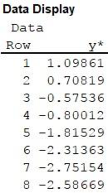
Data transformation
Software procedure:
Step-by-step procedure to transform the data using MINITAB software is given below:
- Choose Calc > Calculator.
- Enter the column of y* under Store result in variable.
- Enter the formula LN(‘p3’/(1–‘p3’)) under Expression.
- Click OK.
The transformed variable is stored in the column y*.
Data display:
Software procedure:
Step by step procedure to display the data using MINITAB software is given as,
- Choose Data > Display Data.
- Under Column, constants, and matrices to display, enter the column of y*.
- Click OK on all dialogue boxes.
The output using MINITAB software is given as follows:
Regression equation:
Software procedure:
Step by step procedure to obtain the regression equation using the MINITAB software:
- Choose Stat > Regression > Regression > Fit Regression Model.
- Enter the column of y* under Responses.
- Enter the columns of x under Continuous predictors.
- Choose Results and select Analysis of Variance, Model Summary, Coefficients, Regression Equation.
- Click OK in all dialogue boxes.
Output obtained using MINITAB is given below:
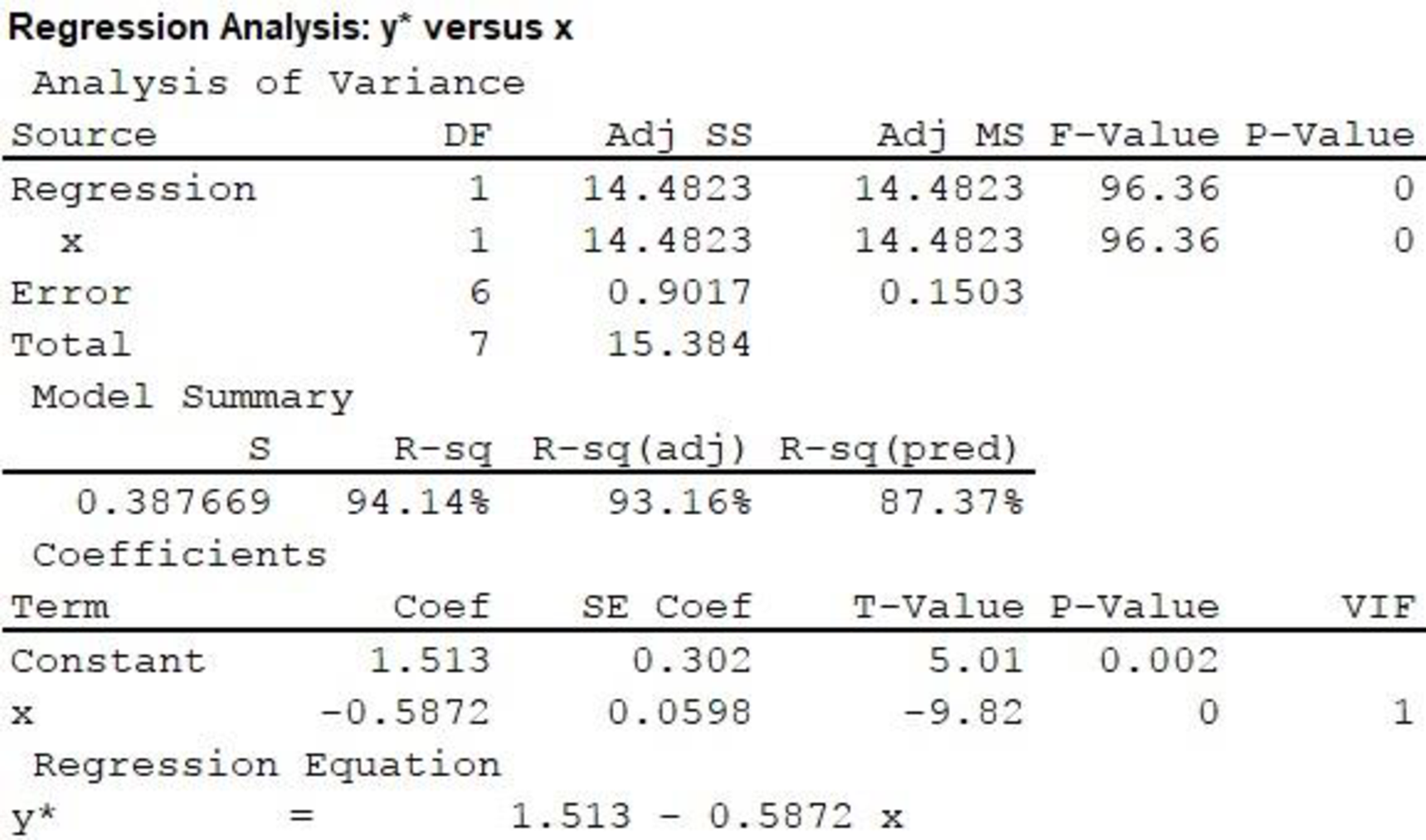
In the output, substituting
It is observed that the slope of x is –0.5872, which is negative. A negative slope implies that an increase in x causes a decrease in yꞌ.
Now, it is known that the quantity
In this case, an increase in exposure time decreases the natural logarithm of odds of hatching in the cloud forest area, which, in turn, implies a decrease in the odds of hatching.
Thus, the negative slope implies that an increase in exposure time causes a decrease in the odds of hatching of an egg in the cloud forest area.
c.
Predict the proportion of hatching in the cloud forest conditions, for an exposure time of 3 days.
Predict the proportion of hatching in the cloud forest conditions, for an exposure time of 5 days.
c.
Answer to Problem 71E
The proportion of hatching in the cloud forest conditions, for an exposure time of 3 days is 0.4382.
The proportion of hatching in the cloud forest conditions, for an exposure time of 5 days is 0.1942.
Explanation of Solution
Calculation:
For an exposure time of 3 days, substitute
Thus,
Thus, the proportion of hatching in the cloud forest conditions, for an exposure time of 3 days is 0.4382.
For an exposure time of 5 days, substitute
Thus,
Thus, the proportion of hatching in the cloud forest conditions, for an exposure time of 5 days is 0.1942.
d.
Identify the point of exposure time, at which, the proportion of hatching in the cloud forest conditions changes from greater than 0.5 to less than 0.5.
d.
Answer to Problem 71E
The exposure time, at which, the proportion of hatching in the cloud forest conditions changes from greater than 0.5 to less than 0.5 is 2.5766 days.
Explanation of Solution
Calculation:
For the proportion of hatching of 0.5, substitute
Thus,
As a result, the exposure time for the proportion of hatching of 0.5 is 2.5766 days.
Now, from the explanation in Part b, an increase in the exposure time causes a decrease in the odds of hatching in the cloud forest conditions. Thus, an increase in exposure time from 2.5766 days would cause a decrease in the proportion of hatching, whereas a decrease in exposure time from 2.5766 days would cause an increase in the proportion of hatching.
Thus, the exposure time, at which, the proportion of hatching in the cloud forest conditions changes from greater than 0.5 to less than 0.5 is 2.5766 days.
Want to see more full solutions like this?
Chapter 5 Solutions
Introduction to Statistics and Data Analysis


- I need help with this problem and an explanation of the solution for the image described below. (Statistics: Engineering Probabilities)arrow_forwardI need help with this problem and an explanation of the solution for the image described below. (Statistics: Engineering Probabilities)arrow_forwardI need help with this problem and an explanation of the solution for the image described below. (Statistics: Engineering Probabilities)arrow_forward
- I need help with this problem and an explanation of the solution for the image described below. (Statistics: Engineering Probabilities)arrow_forwardI need help with this problem and an explanation of the solution for the image described below. (Statistics: Engineering Probabilities)arrow_forward3. Consider the following regression model: Yi Bo+B1x1 + = ···· + ßpxip + Єi, i = 1, . . ., n, where are i.i.d. ~ N (0,0²). (i) Give the MLE of ẞ and σ², where ẞ = (Bo, B₁,..., Bp)T. (ii) Derive explicitly the expressions of AIC and BIC for the above linear regression model, based on their general formulae.arrow_forward
- How does the width of prediction intervals for ARMA(p,q) models change as the forecast horizon increases? Grows to infinity at a square root rate Depends on the model parameters Converges to a fixed value Grows to infinity at a linear ratearrow_forwardConsider the AR(3) model X₁ = 0.6Xt-1 − 0.4Xt-2 +0.1Xt-3. What is the value of the PACF at lag 2? 0.6 Not enough information None of these values 0.1 -0.4 이arrow_forwardSuppose you are gambling on a roulette wheel. Each time the wheel is spun, the result is one of the outcomes 0, 1, and so on through 36. Of these outcomes, 18 are red, 18 are black, and 1 is green. On each spin you bet $5 that a red outcome will occur and $1 that the green outcome will occur. If red occurs, you win a net $4. (You win $10 from red and nothing from green.) If green occurs, you win a net $24. (You win $30 from green and nothing from red.) If black occurs, you lose everything you bet for a loss of $6. a. Use simulation to generate 1,000 plays from this strategy. Each play should indicate the net amount won or lost. Then, based on these outcomes, calculate a 95% confidence interval for the total net amount won or lost from 1,000 plays of the game. (Round your answers to two decimal places and if your answer is negative value, enter "minus" sign.) I worked out the Upper Limit, but I can't seem to arrive at the correct answer for the Lower Limit. What is the Lower Limit?…arrow_forward
- Let us suppose we have some article reported on a study of potential sources of injury to equine veterinarians conducted at a university veterinary hospital. Forces on the hand were measured for several common activities that veterinarians engage in when examining or treating horses. We will consider the forces on the hands for two tasks, lifting and using ultrasound. Assume that both sample sizes are 6, the sample mean force for lifting was 6.2 pounds with standard deviation 1.5 pounds, and the sample mean force for using ultrasound was 6.4 pounds with standard deviation 0.3 pounds. Assume that the standard deviations are known. Suppose that you wanted to detect a true difference in mean force of 0.25 pounds on the hands for these two activities. Under the null hypothesis, 40 0. What level of type II error would you recommend here? = Round your answer to four decimal places (e.g. 98.7654). Use α = 0.05. β = 0.0594 What sample size would be required? Assume the sample sizes are to be…arrow_forwardConsider the hypothesis test Ho: 0 s² = = 4.5; s² = 2.3. Use a = 0.01. = σ against H₁: 6 > σ2. Suppose that the sample sizes are n₁ = 20 and 2 = 8, and that (a) Test the hypothesis. Round your answers to two decimal places (e.g. 98.76). The test statistic is fo = 1.96 The critical value is f = 6.18 Conclusion: fail to reject the null hypothesis at a = 0.01. (b) Construct the confidence interval on 02/2/622 which can be used to test the hypothesis: (Round your answer to two decimal places (e.g. 98.76).) 035arrow_forwardUsing the method of sections need help solving this please explain im stuckarrow_forward
 Algebra & Trigonometry with Analytic GeometryAlgebraISBN:9781133382119Author:SwokowskiPublisher:Cengage
 Functions and Change: A Modeling Approach to Coll...AlgebraISBN:9781337111348Author:Bruce Crauder, Benny Evans, Alan NoellPublisher:Cengage Learning
 Glencoe Algebra 1, Student Edition, 9780079039897...AlgebraISBN:9780079039897Author:CarterPublisher:McGraw Hill