Chapter 4.5, Problem 4E

If X ~ N(2, 9), compute

1. a. P(X ≥ 2)
2. b. P(1 £ X < 7)
3. c. P(–2.5 £ X < –1)
4. d. P(–3 < X –2 < 3)

To determine

Compute the value of $P\left(X\ge 2\right)$.

Answer to Problem 4E

The valueof $P\left(X\ge 2\right)$ is 0.5000.

Explanation of Solution

Given info:

The random variable X is normally distributed with mean $\mu =2$ and variance ${\sigma }^2=9$.

Calculation:

The formula to convert X values into z- score is,

$z=\frac{x-\mu }{\sigma }$

The variance is ${\sigma }^2=9$, thus the standard deviation is,

$\begin{array}{c}\sigma =\sqrt{{\sigma }^2}\\ =\sqrt{9}\\ =3\end{array}$

Now, for $\mu =2$ and $\sigma =3$,

$\begin{array}{c}P\left(X\ge 2\right)=P\left(\frac{X-\mu }{\sigma }>\frac{2-\mu }{\sigma }\right)\\ =P\left(z\ge \frac{2-2}{\sqrt{9}}\right)\\ =P\left(z\ge 0\right)\end{array}$

The value of $P\left(X\ge 2\right)$ is obtained by finding the area to the right of 0.

Use Table A.2: Cumulative Normal Distribution to find the area.

Procedure:

• Locate 0.0 in the left column of the Table A.2.
• Obtain the value in the corresponding row below 0.00.

That is, $P\left(z\ge 0\right)=0.5000$

Software procedure:

Step by step procedure to obtain area under the standard normal curve that lies to the right of $z=-0.85$ using the MINITAB software:

• Choose Graph > Probability Distribution Plot >View Single, and then clickOK.
• From Distribution, choose ‘Normal’ distribution.
• Under Mean, enter 0.
• Under Standard deviation, enter 1.
• Click the Shaded Area tab.
• Choose X Value and right tail for the region of the curve to shade.
• Enter the value as 0.
• Click OK.

Output using MINITAB software is given below:

The shaded region represents the area to the right of 0.

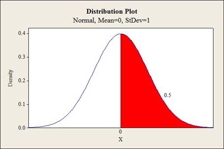
Thus, the value of $P\left(X\ge 2\right)$ is 0.5000.

To determine

Compute the value of $P\left(1\le X<7\right)$.

Answer to Problem 4E

The value of $P\left(1\le X<7\right)$ is 0.5818.

Explanation of Solution

Calculation:

Now, for $\mu =2$ and $\sigma =3$,

$\begin{array}{c}P\left(1\le X<7\right)=P\left(\frac{1-\mu }{\sigma }\le \frac{X-\mu }{\sigma }<\frac{7-\mu }{\sigma }\right)\\ =P\left(\frac{1-2}{3}\le z<\frac{7-2}{3}\right)\\ =P\left(\frac{-1}{3}\le z\le \frac{5}{3}\right)\\ =P\left(-0.33\le z\le 1.67\right)\end{array}$

The value of $P\left(1\le X<7\right)$ is obtained by finding the difference between the area the left of 1.67 and to the left of –0.33.

Use Table A.2: Standard normal (z) distribution to find the areas.

Procedure:

For z at 1.67,

• Locate 1.6 in the left column of the TableA.2.
• Obtain the value in the corresponding row below 0.07.

That is, $P\left(z\le 1.67\right)=0.9525$

For z at –0.33,

• Locate –0.3 in the left column of the Table A.2.
• Obtain the value in the corresponding row below 0.03.

That is, $P\left(z\le -0.33\right)=0.3707$

The difference between the areas is,

$\begin{array}{c}P\left(-0.33\le X\le 1.67\right)=P\left(X\le 1.67\right)-P\left(X\le -0.33\right)\\ =0.9525-0.3707\\ =0.5818\end{array}$

Software procedure:

Step by step procedure to obtain area under the standard normal curve that lies between $z=-0.33$ and $z=1.67$ using the MINITAB software:

• Choose Graph > Probability Distribution Plot >View Single, and then clickOK.
• From Distribution, choose ‘Normal’ distribution.
• Under Mean, enter 0.
• Under Standard deviation, enter 1.
• Click the Shaded Area tab.
• Choose X Value and middle for the region of the curve to shade.
• Enter the value as –0.33 and 1.67.
• Click OK.

Output using MINITAB software is given below:

The shaded region represents the area between $z=-0.33$ and $z=1.67$.

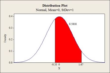
Thus, the value of probability is $\underset{\_}{P\left(-0.33\le X\le 1.67\right)=0.5818}$.

To determine

Compute the value of $P\left(-2.5\le X<-1\right)$.

Answer to Problem 4E

The value of $P\left(-2.5\le X<-1\right)$ is 0.0919.

Explanation of Solution

Calculation:

Now, for $\mu =2$ and $\sigma =3$,

$\begin{array}{c}P\left(-2.5\le X<-1\right)=\left(\frac{-2.5-\mu }{\sigma }\le \frac{X-\mu }{\sigma }<\frac{-1-\mu }{\sigma }\right)\\ =P\left(\frac{-2.5-2}{3}\le z<\frac{-1-2}{3}\right)\\ =P\left(\frac{-4.5}{3}\le z\le \frac{-3}{3}\right)\\ =P\left(-1.5\le z\le -1\right)\end{array}$

The value of $P\left(-2.5\le X<-1\right)$ is obtained by finding the difference between the area the left of –1 and to the left of –1.5.

Use Table A.2: Standard normal (z) distribution to find the areas.

Procedure:

For z at –1.00,

• Locate –1.0 in the left column of the TableA.2.
• Obtain the value in the corresponding row below 0.00.

That is, $P\left(z\le -1.00\right)=0.1587$

For z at –1.5,

• Locate –1.5 in the left column of the Table A.2.
• Obtain the value in the corresponding row below 0.00.

That is, $P\left(z\le -1.5\right)=0.0668$

The difference between the areas is,

$\begin{array}{c}P\left(-2.5\le X<-1\right)=P\left(z\le -1.00\right)-P\left(z\le -1.50\right)\\ =0.1587-0.0668\\ =0.0919\end{array}$

Software procedure:

Step by step procedure to obtain area under the standard normal curve that lies between $z=-2.5$ and $z=-1$ using the MINITAB software:

• Choose Graph > Probability Distribution Plot >View Single, and then clickOK.
• From Distribution, choose ‘Normal’ distribution.
• Under Mean, enter 0.
• Under Standard deviation, enter 1.
• Click the Shaded Area tab.
• Choose X Value and middle for the region of the curve to shade.
• Enter the value as –2.5 and –1.
• Click OK.

Output using MINITAB software is given below:

The shaded region represents the area between $z=-2.5$ and $z=-1$.

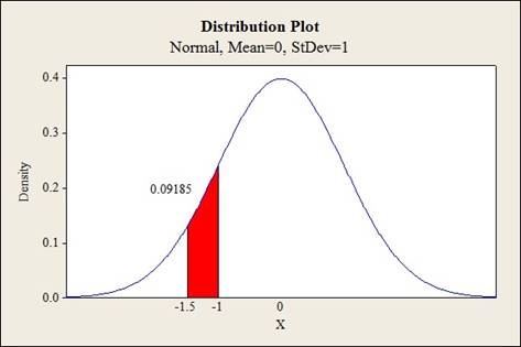
Thus, the value of probability is $\underset{\_}{P\left(-2.5\le X<-1\right)=0.0919}$.

To determine

Compute the value of $P\left(-3\le X-2<3\right)$.

Answer to Problem 4E

The value of $P\left(-3\le X-2<3\right)$ is 0.6826.

Explanation of Solution

Calculation:

Now, for $\mu =2$ and $\sigma =3$,

$\begin{array}{c}P\left(-3\le X-2<3\right)=P\left(-1\le X<5\right)\\ =P\left(\frac{-1-\mu }{\sigma }\le \frac{X-\mu }{\sigma }<\frac{5-\mu }{\sigma }\right)\\ =P\left(\frac{-1-2}{3}\le z<\frac{5-2}{3}\right)\\ =P\left(\frac{-3}{3}\le z\le \frac{3}{3}\right)\end{array}$

$=P\left(-1\le z\le 1\right)$

The value of $P\left(-3\le X-2<3\right)$ is obtained by finding the difference between the area the left of 1 and to the left of –1.

Use Table A.2: Standard normal (z) distribution to find the areas.

Procedure:

For z at 1.00,

• Locate 1.0 in the left column of the TableA.2.
• Obtain the value in the corresponding row below 0.00.

That is, $P\left(z\le 1.00\right)=0.8413$

For z at –1.00,

• Locate –1.0 in the left column of the Table A.2.
• Obtain the value in the corresponding row below 0.00.

That is, $P\left(z\le -1.00\right)=0.1587$

The difference between the areas is,

$\begin{array}{c}P\left(-3\le X-2<3\right)=P\left(z\le 1.00\right)-P\left(z\le -1.00\right)\\ =0.8413-0.1587\\ =0.6826\end{array}$

Software procedure:

Step by step procedure to obtain area under the standard normal curve that lies between $z=-1$ and $z=1$ using the MINITAB software:

• Choose Graph > Probability Distribution Plot >View Single, and then click OK.
• From Distribution, choose ‘Normal’ distribution.
• Under Mean, enter 0.
• Under Standard deviation, enter 1.
• Click the Shaded Area tab.
• Choose X Value and middle for the region of the curve to shade.
• Enter the value as –1 and 1.
• Click OK.

Output using MINITAB software is given below:

The shaded region represents the area between $z=-1$ and $z=1$.

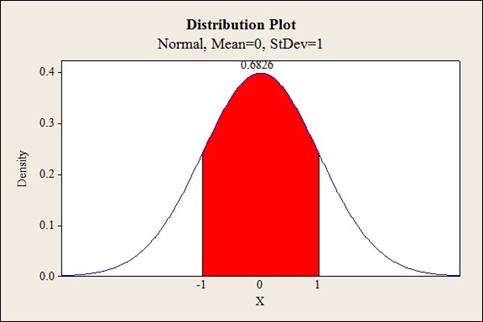
Thus, the value of probability is $\underset{\_}{P\left(-3\le X-2<3\right)=0.6826}$.