Concept explainers
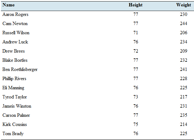
Pass the ball: The following table lists the heights (inches) and weights (pounds) of 14 National Football League quarterbacks in the 2016 season.

- Compute the least-squares regression line for predicting weight from height.
- Is it possible to interpret the y-intercept? Explain.
- If two quarterbacks differ in height by two inches: by how much would you predict their weights to differ?
- Predict the of a quarterback who is 74.5 inches tall.
- Kirk Cousins is 75 inches tall and weighs 214 pounds. Does he weigh more or less than the weight predicted by the least-squares regression line?
a.
To find: The least-square regression line for the given data set.
Answer to Problem 23E
The least square regression line of the given data set is,
Explanation of Solution
Following table with the heights and the weights of the national football quarterbacks in the season
| Name | Height | Weight |
| Aaron Rogers | 77 | 230 |
| Cam Newton | 77 | 244 |
| Russell Wilson | 71 | 206 |
| Andrew Luck | 76 | 234 |
| Drew Brees | 72 | 209 |
| Blake Bortles | 77 | 232 |
| Ben Roethlisberger | 77 | 241 |
| Philip Rivers | 77 | 228 |
| Eli Manning | 76 | 225 |
| Tyrod Taylor | 73 | 217 |
| Jamies Winston | 76 | 231 |
| Carson Palmer | 77 | 235 |
| Kirk Cousins | 75 | 214 |
| Tom Brady | 76 | 225 |
Calculation:
The least-square regression is given by the formula,
Where
The correlation coefficient is given by the formula,
Let

The correlation coefficient can be obtained by the following table.
Hence, the correlation coefficient is,
Then, the coefficient
Therefore,
Conclusion:
The least square regression line is found to be,
b.
To explain:The possibility to interpret the
Answer to Problem 23E
The
Explanation of Solution
The least-square regression line has been computed as
Considering the
The
Conclusion:
There is no chance to a weight be a negative value. Therefore, this
c.
To calculate:The difference in the weight of two players when their heights differ by two inches.
Answer to Problem 23E
The difference of weight is found to be
Explanation of Solution
The least-square regression line has been computed as
Calculation:
Let the height of the shorter payer be
Also, the weight of the taller player should be,
Simplifying the obtained weight,
Therefore, the difference of two weights should be,
Interpretation:
As the calculation above, the weight difference for two inches change in the height is found to be
d.
To find:The predicted weight of a player whose height is
Answer to Problem 23E
The weight of a player whose height is
Explanation of Solution
Calculation:
By the computed least-square regression line, we can calculate the predictions for the weights of the players by substituting their heights into the formula.
Here, the height is said to be
Conclusion:
The weight of a player whose height is
e.
To find:Whether theactual weight of this player is greater than the predicted weight or not.
Answer to Problem 23E
The player weighs less than the predicted weight.
Explanation of Solution
The player is
Calculation:
When the height is said to be
The predicted weight is found to be
Conclusion:
Since
Want to see more full solutions like this?
Chapter 4 Solutions
Elementary Statistics
- The following table shows a data set containing information for 25 of the shadow stocks tracked by the American Association of Individual Investors (aaii.com, February 2002). Shadow stocks are common stocks of smaller companies that are not closely followed by Wall Street analysts. Click on the datafile logo to reference the data. DATA file Company DeWolfe Companies Exchange AMEX Ticker Symbol Market Cap Price/ Gross Profit Earnings Margin ($ millions) Ratio (%) DWL 36.4 8.4 36.7 North Coast Energy OTC NCEB 52.5 6.2 59.3 Hansen Natural Corp. OTC HANS 41.1 14.6 44.8 MarineMax, Inc. NYSE HZO 111.5 7.2 23.8 Nanometrics Incorporated OTC NANO 228.6 38.0 53.3 TeamStaff, Inc. OTC TSTF 92.1 33.5 4.1 Environmental Tectonics AMEX ETC 51.1 35.8 35.9 Measurement Specialties AMEX MSS 101.8 26.8 37.6 SEMCO Energy, Inc. NYSE SEN 193.4 18.7 23.6 Party City Corporation OTC PCTY 97.2 15.9 36.4 Embrex, Inc. OTC EMBX 136.5 18.9 59.5 Tech/Ops Sevcon, Inc. AMEX ΤΟ 23.2 20.7 35.7 ARCADIS NV OTC ARCAF 173.4…arrow_forwardThe following data show the year to date percent change (YTD % Change) for 30 stock-market indexes from around the word (The Wall Street Journal, August 26, 2013). a. What index has the largest positive YTD % Change? Round your answer to once decimal place. index with a YTD % Change of % b. Using a class width of 5 beginning with -20 and going to 40, develop a frequency distribution for the data. YTD % Change Frequency -20 - -15 -15 - -10 -10 - -5 -5 - 0 0 - 5 5 - 10 10 - 15 15 - 20 20 - 25 30 - 35 c. 1. 2. 3. 4.arrow_forwardThe following data show the year to date percent change (YTD % Change) for 30 stock-market indexes from around the word (The Wall Street Journal, August 26, 2013). Click on the datafile logo to reference the data. DATA file Country Australia Index S&P/ASX200 YTD % Change 10.2 Belgium Bel-20 12.6 Brazil São Paulo Bovespa -14.4 Canada S&P/TSX Comp 2.6 Chile Santiago IPSA -16.3 China Shanghai Composite -9.3 Eurozone EURO Stoxx 10.0 France CAC 40 11.8 Germany DAX 10.6 Hong Kong Hang Seng -3.5 India S&P BSE Sensex -4.7 Israel Tel Aviv 1.3 Italy FTSE MIB 6.6 Japan Nikkei 31.4 Mexico IPC All-Share -6.4 Netherlands AEX 9.3 Singapore Straits Times -2.5 South Korea Kospi -6.4 Spain IBEX 35 6.4 Sweden Switzerland SX All Share 13.8 Swiss Market 17.4 Taiwan Weighted 2.3 U.K. FTSE 100 10.1 U.S. S&P 500 16.6 U.S. DJIA 14.5 U.S. Dow Jones Utility 6.6 U.S. Nasdaq 100 17.4 U.S. Nasdaq Composite 21.1 World DJ Global ex U.S. 4.2 World DJ Global Index 9.9 a. What index has the largest positive YTD %…arrow_forward
- Describe a three step process you choose to determine how many elementary schools there are in the city of 5 million people.arrow_forwardQuiz: Exam 1 (Ch 1-4) z Scores Table-3.pdf x + edu/courses/308627/quizzes/2442507/take/questions/48957332 Canvas Hall It browser 5 Connect Set as default incorrect. • This exam is NOT resumable. Meaning, once you start the exam, you must complete it in its entirety. Any blank questions will be marked as By taking this exam, you agree to adhere to the academic integrity standards, which consist of NOT cheating in any way. To get the highest possible score, you are encouraged to review your notes before taking the exam. You may use your notes during the exam, but note that you should be familiar with the concepts and formulas before taking exam. z Scores Table.pdf Question 3 3 pts Here is a data from a survey asking young children how many hours they spend playing video games. The researchers reported the percent of boys and girls who played no games, less than 1 hour per day, 1-3 hours per day, or greater than 3 hours per day. The most common number of hours per day that boys played is…arrow_forwardWrite a Regression summary explaining significance of mode, explaining regression coefficients, significance of the independent variables, R and R square. Premiums earned Net income Dividends Underwriting Gain/ Loss 30.2 1.6 0.6 0.1 47.2 0.6 0.7 -3.6 92.8 8.4 1.8 -1.5 95.4 7.6 2 -4 100.4 6.3 2.2 -8.1 104.9 6.3 2.4 -10.8 113.2 2.2 2.3 -18.2 130.3 3.0 2.4 -21.4 161.9 13.5 2.3 -12.8 182.5 14.9 2.9 -5.9 193.3 11.7 2.9 -7.6arrow_forward
- 1- Let A = {A1, A2, ...), in which A, A, = 0, when i j. a) Is A a π-system? If not, which element(s) should be added to A to become a π-system? b) Prove that σ(A) consists of the finite or countable unions of elements of A; i.c., A E σ(A) if and only if there exists finite or countable sequence {n} such that A = U₁An (Hint: Let F be such class; prove that F is a σ-filed containing A.) c) Let p ≥ 0 be a sequence of non-negative real numbers with Σip₁ = 1. Using p₁'s, how do you construct a probability measure on σ(A)? (Hint: use extension theorem.) 2- Construct an example for which P(lim sup A,) = 1 and P(lim inf An) = 0.arrow_forwardIn a town with 5000 adults, a sample of 50 is selected using SRSWOR and asked their opinion of a proposed municipal project; 30 are found to favor it and 20 oppose it. If, in fact, the adults of the town were equally divided on the proposal, what would be the probability of observing what has been observed? Approximate using the Binomial distribution. Compare this with the exact probability which is 0.0418.arrow_forwardGood explanation it sure experts solve itarrow_forward
- Best explains it not need guidelines okkarrow_forwardActiv Determine compass error using amplitude (Sun). Minimum number of times that activity should be performed: 3 (1 each phase) Sample calculation (Amplitude- Sun): On 07th May 2006 at Sunset, a vessel in position 10°00'N 010°00'W observed the Sun bearing 288° by compass. Find the compass error. LMT Sunset: LIT: (+) 00d 07d 18h 00h 13m 40m UTC Sunset: 07d 18h 53m (added- since longitude is westerly) Declination (07d 18h): N 016° 55.5' d (0.7): (+) 00.6' Declination Sun: N 016° 56.1' Sin Amplitude = Sin Declination/Cos Latitude = Sin 016°56.1'/ Cos 10°00' = 0.295780189 Amplitude=W17.2N (The prefix of amplitude is named easterly if body is rising, and westerly if body is setting. The suffix is named same as declination) True Bearing=287.2° Compass Bearing= 288.0° Compass Error = 0.8° Westarrow_forwardOnly sure experts solve it correct complete solutions okkarrow_forward
 Glencoe Algebra 1, Student Edition, 9780079039897...AlgebraISBN:9780079039897Author:CarterPublisher:McGraw Hill
 Big Ideas Math A Bridge To Success Algebra 1: Stu...AlgebraISBN:9781680331141Author:HOUGHTON MIFFLIN HARCOURTPublisher:Houghton Mifflin Harcourt
 Holt Mcdougal Larson Pre-algebra: Student Edition...AlgebraISBN:9780547587776Author:HOLT MCDOUGALPublisher:HOLT MCDOUGAL
 Functions and Change: A Modeling Approach to Coll...AlgebraISBN:9781337111348Author:Bruce Crauder, Benny Evans, Alan NoellPublisher:Cengage Learning


