Concept explainers
Videos
Presidents and first ladies: The presents the ages of the last 10 U.S. presidents and their wives on the first day of their presidencies.
- Compute the least-squares regression line for predicting the president’s age from the first lady’s age.
- Compute the coefficient of determination-
- Construct a
scatterplot of the presidents' ages (y) versus the first ladies' ages (x). - Which point is an outlier?
- Remove die outlier and compute the least-squares regression line for predicting the president’s age from the first lady: s age.
- Is the outlier influential? Explain.
- Compute the coefficient of determination for the data set with the outlier removed. Is due proportion of variation explained by due least-squares regression he greater, less. or about the same without due outlier? Explain.
a.
To Calculate: The least-squares regression line for predicting the president’s age from lady’s age.
Answer to Problem 24E
The least-squares regression line is,
ˆy=14+0.8426x
Explanation of Solution
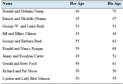
Given: The following table presents the age of the president’s and their wives on the first day of their presidencies.
| Name | Her Age | His Age |
| Donald and Melania Trump | 46 | 70 |
| Barak and Mechelle Obama | 45 | 47 |
| George W. and Laura Bush | 54 | 54 |
| Bill and Hillary Clinton | 45 | 46 |
| George and Babara Bush | 55 | 64 |
| Ronald and Nancy Reagan | 59 | 69 |
| Jimmy and Rosalyn Carter | 49 | 52 |
| Gerald and Betty Ford | 56 | 61 |
| Richard and Pat Nixon | 56 | 56 |
| Lyndon and Lady Bird Johnson | 50 | 55 |
Calculation:
Here,
y = president’s age
x = lady’s age
From below formula we can find least regression line.
ˆy=b0+b1x
where b0 and b1 are constants.
We can find these constants from below formulas.
b1=rsysxb0=ˉy−b1ˉxr=1n−1∑(x−ˉxsx)(y−ˉysy)
Where,
n is the number of observations
ˉx is the average of x
ˉy is the average of y
sx is the standard deviation of x
sy is the standard deviation of y
| Descriptive Statistics | |||
| N | Mean | Std. Deviation | |
| His age | 10 | 57.40 | 8.409 |
| Her age | 10 | 51.50 | 5.148 |
| Valid N (listwise) | 10 | ||
n=10 number of observations
ˉx=51.5 average of lady’s age (x)
ˉy=57.4 average of president’s age (y)
sx=5.148 standard deviation of x
sy=8.409 standard deviation of y
r=0.5159 correlation between x and y
To find constants,
b1=rsysxb1=0.5159×8.4095.148 =0.8426
And,
b0=ˉy−b1ˉx =57.4−(0.8426×51.5) b0=14.0061b0≈14
By substituting above formula,
y=b0+b1xy=14+0.8426x
Conclusion:
The least-squares regression line for predicting the president’s age from lady’s age is,
y=14+0.8426x
b.
To find: The correlation coefficient of the two variables.
Answer to Problem 24E
The correlation coefficient is found to be,
r=0.5159
Explanation of Solution
Calculation:
The correlation coefficient (r) is given by the formula,
r=1n−1∑(x−ˉxsx)(y−ˉysy)
Where sx and sy is the standard deviation of x and y .
The means and the standard deviations of the both variables can be obtained by using the Excel.
| Descriptive Statistics | |||
| N | Mean | Std. Deviation | |
| His age | 10 | 57.40 | 8.409 |
| Her age | 10 | 51.50 | 5.148 |
| Valid N (listwise) | 10 | ||
Then,
ˉx=51.5sx=5.148ˉy=57.4sy=8.409
Then, a table should be constructed to calculate r as follows.
Her AgexHis Ageyx−ˉxsxy−ˉysy(x−ˉxsx)(y−ˉysy)4670−1.06841.4984−1.60094547−1.2626−1.23681.561654540.4856−0.4043−0.19634546−1.2626−1.35571.711755640.67990.78490.533759691.45691.37952.00984952−0.4856−0.64220.311956610.87410.42810.374256560.8741−0.1665−0.14555055−0.2914−0.28540.0832∑(x−ˉxsx)(y−ˉysy)=4.6434
The correlation coefficient can be calculated as,
r=110−1×4.6434=4.64349r=0.5159
Conclusion:
The correlation coefficient between the interest rates for two mortgage plans is found tobe,
r=0.5159
c.
To graph: The scatter plot of the given two quantitative variables.
Explanation of Solution
Graph:
Let x be the lady’s age and y be the president’s age. The scatter plot can be constructed by the ordered pairs using the Excel.
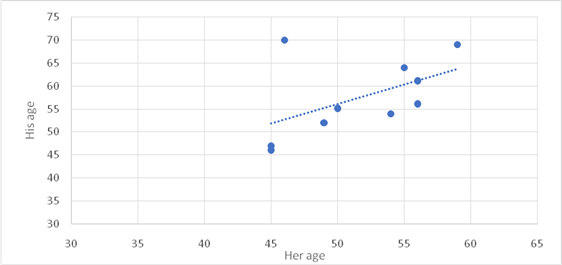
Interpretation:
Out of all these 10 ordered pairs, there is a weak positive relationship between president’s age and lady’s age.
d.
To Identify: The outliers within the given data.
Answer to Problem 24E
There is one outlier which is age 70
Explanation of Solution
Explain:
Here, Excel is used to calculate below statistics.
Q1 is the middle value in the first half of the rank-ordered data set.
Q2 is the median value in the set.
Q3 is the middle value in the second half of the rank-ordered data set.
The interquartile range is equal to Q3 minus Q1 .
To calculate upper bound,
Q3+(IQR×1.5)=Q3+((Q3−Q1)×1.5)=56.75+(56.75−48.5)×1.5=56.75+8.25×1.5=56.75+12.375Q3+(IQR×1.5)=69.125
To calculate lower bound,
Q1−(IQR×1.5)=Q1−((Q3−Q1)×1.5)=48.5−(56.75−48.5)×1.5=48.5−8.25×1.5=48.5−12.375Q1−(IQR×1.5)=36.125
An outlier is a data point that lies outside the upper bound and lower bound.
Q1Q3IQRLower BoundUpperBound48.556.758.2536.12569.125
Out of all 10 ordered pairs, only one value can be identified as an outlier, where the age is not between the lower bound and upper bound.
70>69.125
e.
To find: The least-squares regression line for predicting the president’s age from lady’s age with removing outlier.
Answer to Problem 24E
The least-squares regression is,
y=−14.7+1.3567x
Explanation of Solution
Calculation:
Here,
y = president’s age
x = lady’s age
From below formula we can find least regression line.
ˆy=b0+b1x
where b0 and b1 are constants.
We can find constants from below formulas.
b1=rsysxb0=ˉy−b1ˉxr=1n−1∑(x−ˉxsx)(y−ˉysy)
Where,
n is the number of observationsˉx is the average of x
ˉy is the average of y
sx is the standard deviation of x
sy is the standard deviation of y
When the outlier is removed, the number of ordered pairs is 9 .
| Descriptive Statistics | |||
| N | Mean | Std. Deviation | |
| His age | 9 | 56.00 | 7.583 |
| Her age | 9 | 52.11 | 5.061 |
| Valid N (listwise) | 9 | ||
n=9 ; number of observations.
ˉx=52.11 ; average of lady’s age (x)
ˉy=56 ; average of president’s age (y)
sx=5.061 ; standard deviation of x
sy=7.583 ; standard deviation of y
r=0.9055 ; correlation between x and y
To find constants,
b1=rsysxb1=(0.9055)7.5835.061 =1.3567
And,
b0=ˉy−b1ˉx =56−(1.3567)×52.11 =−14.6976 =−14.7
By substituting into the above formula,
y=b0+b1xy=−14.7+1.3567x
Conclusion:
The least-squares regression line for predicting the president’s age from lady’s age is,
y=−14.7+1.3567x
f.
To Check: The influence of outlier.
Answer to Problem 24E
Yes. It is influenced.
Explanation of Solution
Explain:
| Descriptive Statistics | |||
| N | Mean | Std. Deviation | |
| His age | 10 | 57.40 | 8.409 |
| Her age | 10 | 51.50 | 5.148 |
| Valid N (listwise) | 10 | ||
| Descriptive Statistics | |||
| N | Mean | Std. Deviation | |
| His age | 9 | 56.00 | 7.583 |
| Her age | 9 | 52.11 | 5.061 |
| Valid N (listwise) | 9 | ||
To calculate above statistics, Excel is used. Here we can see statistics with outlier and without outlier. Second table shows statistics without outlier. Total number of observations, mean and standard deviation of dependent and independent variables are changed. So, it influences to least squares regression line for predicting the president’s age from lady’s age.
g.
To find: The correlation coefficient of the two variables without outlier.
Answer to Problem 24E
The correlation coefficient is found to be,
r=0.9055
Explanation of Solution
Calculation:
The correlation coefficient (r) is given by the formula,
r=1n−1∑(x−ˉxsx)(y−ˉysy)
Where sx and sy is the standard deviation of x and y .
The means and the standard deviations of the both variables can be obtained by using the Excel.
For the remaining 9 pairs without the outlier,
| Descriptive Statistics | |||
| N | Mean | Std. Deviation | |
| His age | 9 | 56.00 | 7.583 |
| Her age | 9 | 52.11 | 5.061 |
| Valid N (listwise) | 9 | ||
Then,
ˉx=52.11sx=5.061ˉy=56sy=7.583
Then, a table should be constructed to calculate r as follows.
xyx−ˉxsxy−ˉysy(x−ˉxsx)(y−ˉysy)4547−1.4051−1.18691.667754540.3732−0.2637−0.09844546−1.4051−1.31871.852955640.57081.05500.602259691.36121.71442.33364952−0.6147−0.52750.324356610.76840.65940.506756560.7684005055−0.4171−0.13190.0550∑(x−ˉxsx)(y−ˉysy)=7.2438
The correlation coefficient can be calculated as,
r=19−1×7.2438=7.24388r=0.9055
Conclusion:
The correlation coefficient between the interest rates for two mortgage plans is found to be,
r=0.9055
Want to see more full solutions like this?
Chapter 4 Solutions
Elementary Statistics


- The acidity or alkalinity of a solution is measured using pH. A pH less than 7 is acidic; a pH greater than 7 is alkaline. The accompanying data represent the pH in samples of bottled water and tap water. Complete parts (a) and (b). Click the icon to view the data table. (a) Determine the mean, median, and mode pH for each type of water. Comment on the differences between the two water types. Select the correct choice below and fill in any answer boxes in your choice. A. For tap water, the mean pH is (Round to three decimal places as needed.) B. The mean does not exist. Data table Тар 7.64 7.45 7.45 7.10 7.46 7.50 7.68 7.69 7.56 7.46 7.52 7.46 5.15 5.09 5.31 5.20 4.78 5.23 Bottled 5.52 5.31 5.13 5.31 5.21 5.24 - ☑arrow_forwardく Chapter 5-Section 1 Homework X MindTap - Cengage Learning x + C webassign.net/web/Student/Assignment-Responses/submit?pos=3&dep=36701632&tags=autosave #question3874894_3 M Gmail 品 YouTube Maps 5. [-/20 Points] DETAILS MY NOTES BBUNDERSTAT12 5.1.020. ☆ B Verify it's you Finish update: All Bookmarks PRACTICE ANOTHER A computer repair shop has two work centers. The first center examines the computer to see what is wrong, and the second center repairs the computer. Let x₁ and x2 be random variables representing the lengths of time in minutes to examine a computer (✗₁) and to repair a computer (x2). Assume x and x, are independent random variables. Long-term history has shown the following times. 01 Examine computer, x₁₁ = 29.6 minutes; σ₁ = 8.1 minutes Repair computer, X2: μ₂ = 92.5 minutes; σ2 = 14.5 minutes (a) Let W = x₁ + x2 be a random variable representing the total time to examine and repair the computer. Compute the mean, variance, and standard deviation of W. (Round your answers…arrow_forwardThe acidity or alkalinity of a solution is measured using pH. A pH less than 7 is acidic; a pH greater than 7 is alkaline. The accompanying data represent the pH in samples of bottled water and tap water. Complete parts (a) and (b). Click the icon to view the data table. (a) Determine the mean, median, and mode pH for each type of water. Comment on the differences between the two water types. Select the correct choice below and fill in any answer boxes in your choice. A. For tap water, the mean pH is (Round to three decimal places as needed.) B. The mean does not exist. Data table Тар Bottled 7.64 7.45 7.46 7.50 7.68 7.45 7.10 7.56 7.46 7.52 5.15 5.09 5.31 5.20 4.78 5.52 5.31 5.13 5.31 5.21 7.69 7.46 5.23 5.24 Print Done - ☑arrow_forward
- The median for the given set of six ordered data values is 29.5. 9 12 23 41 49 What is the missing value? The missing value is ☐.arrow_forwardFind the population mean or sample mean as indicated. Sample: 22, 18, 9, 6, 15 □ Select the correct choice below and fill in the answer box to complete your choice. O A. x= B. μεarrow_forwardWhy the correct answer is letter A? Students in an online course are each randomly assigned to receive either standard practice exercises or adaptivepractice exercises. For the adaptive practice exercises, the next question asked is determined by whether the studentgot the previous question correct. The teacher of the course wants to determine whether there is a differencebetween the two practice exercise types by comparing the proportion of students who pass the course from eachgroup. The teacher plans to test the null hypothesis that versus the alternative hypothesis , whererepresents the proportion of students who would pass the course using standard practice exercises andrepresents the proportion of students who would pass the course using adaptive practice exercises.The teacher knows that the percent confidence interval for the difference in proportion of students passing thecourse for the two practice exercise types (standard minus adaptive) is and the percent…arrow_forward
- Carpetland salespersons average $8,000 per week in sales. Steve Contois, the firm's vice president, proposes a compensation plan with new selling incentives. Steve hopes that the results of a trial selling period will enable him to conclude that the compensation plan increases the average sales per salesperson. a. Develop the appropriate null and alternative hypotheses.H 0: H a:arrow_forwardتوليد تمرين شامل حول الانحدار الخطي المتعدد بطريقة المربعات الصغرىarrow_forwardThe U.S. Postal Service will ship a Priority Mail® Large Flat Rate Box (12" 3 12" 3 5½") any where in the United States for a fixed price, regardless of weight. The weights (ounces) of 20 ran domly chosen boxes are shown below. (a) Make a stem-and-leaf diagram. (b) Make a histogram. (c) Describe the shape of the distribution. Weights 72 86 28 67 64 65 45 86 31 32 39 92 90 91 84 62 80 74 63 86arrow_forward
- (a) What is a bimodal histogram? (b) Explain the difference between left-skewed, symmetric, and right-skewed histograms. (c) What is an outlierarrow_forward(a) Test the hypothesis. Consider the hypothesis test Ho = : against H₁o < 02. Suppose that the sample sizes aren₁ = 7 and n₂ = 13 and that $² = 22.4 and $22 = 28.2. Use α = 0.05. Ho is not ✓ rejected. 9-9 IV (b) Find a 95% confidence interval on of 102. Round your answer to two decimal places (e.g. 98.76).arrow_forwardLet us suppose we have some article reported on a study of potential sources of injury to equine veterinarians conducted at a university veterinary hospital. Forces on the hand were measured for several common activities that veterinarians engage in when examining or treating horses. We will consider the forces on the hands for two tasks, lifting and using ultrasound. Assume that both sample sizes are 6, the sample mean force for lifting was 6.2 pounds with standard deviation 1.5 pounds, and the sample mean force for using ultrasound was 6.4 pounds with standard deviation 0.3 pounds. Assume that the standard deviations are known. Suppose that you wanted to detect a true difference in mean force of 0.25 pounds on the hands for these two activities. Under the null hypothesis, 40 = 0. What level of type II error would you recommend here? Round your answer to four decimal places (e.g. 98.7654). Use a = 0.05. β = i What sample size would be required? Assume the sample sizes are to be equal.…arrow_forward
 Glencoe Algebra 1, Student Edition, 9780079039897...AlgebraISBN:9780079039897Author:CarterPublisher:McGraw Hill
 Big Ideas Math A Bridge To Success Algebra 1: Stu...AlgebraISBN:9781680331141Author:HOUGHTON MIFFLIN HARCOURTPublisher:Houghton Mifflin Harcourt
 Holt Mcdougal Larson Pre-algebra: Student Edition...AlgebraISBN:9780547587776Author:HOLT MCDOUGALPublisher:HOLT MCDOUGAL
 Linear Algebra: A Modern IntroductionAlgebraISBN:9781285463247Author:David PoolePublisher:Cengage Learning
 Elementary Linear Algebra (MindTap Course List)AlgebraISBN:9781305658004Author:Ron LarsonPublisher:Cengage Learning