Concept explainers
Videos
(a)
The
(a)
Answer to Problem 23P
Solution: The provided values, that is,
Explanation of Solution
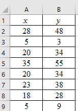
Given: The provided table consists of values of x and y, where x represents the average annual hours spent by a person in traffic delay, y represents the average annual gallons of fuel wasted per person due to traffic delay. The data consists of 8 data pairs, thus n is 8.
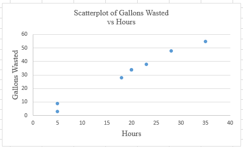
Calculation: Follow the steps given below in MS Excel to obtain the scatter plot of the data.
Step 1: Enter the data into an MS Excel sheet. The screenshot is given below.
Step 2: Select the data and click on ‘Insert’. Go to charts and select the chart type ‘Scatter’.

Step 3: Select the first plot and then click ‘add chart element’ provided in the left corner of the menu bar. Insert the ‘Axis titles’ and ‘Chart title’. The scatter plot for the provided data is shown below:
To calculate
| 28 | 48 | 784 | 2304 | 1344 |
| 5 | 3 | 25 | 9 | 15 |
| 20 | 34 | 400 | 1156 | 680 |
| 35 | 55 | 1225 | 3025 | 1925 |
| 20 | 34 | 400 | 1156 | 680 |
| 23 | 38 | 529 | 1444 | 874 |
| 18 | 28 | 324 | 784 | 504 |
| 5 | 9 | 25 | 81 | 45 |
The provided values,
Now, the value of
Substituting the values in the above formula. Thus:
Therefore, the correlation coefficient is 0.991.
(b)
The averages
(b)
Answer to Problem 23P
Solution: The values for data set 1 are
The values for data set 2 are
Explanation of Solution
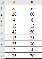
Given: The provided table consists of values of x and y, where x represents the average annual hours spent by a person in traffic delay, y represents the average annual gallons of fuel wasted per person due to traffic delay.
The second table consists of x and y values where, x represent the annual hours lost by a person spent in traffic delay, y represents the annual gallons of fuel wasted by that person in traffic delay.
The data sets consist of 8 data pairs, thus n is 8 for both the data sets.
The provided values of data set 1 are,
The provided values of data set 2 are,
Calculation:
The value of
The value of
The standard deviation of x for data set 1 can be calculated as,
The standard deviation of
The value of
The value of
The standard deviation of
The standard deviation of
For the second data set, that is, for the variables based on single individuals, the standard deviations
The values
(c)
The scatter plot, whether the provided values of
(c)
Answer to Problem 23P
Solution: The provided values, that is,
Explanation of Solution
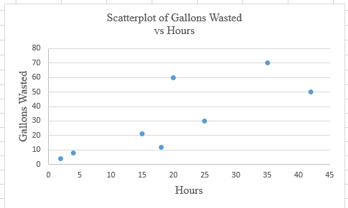
The provided table consists of values of x and y, where x represents the average annual hours spent by a person in traffic delay, y represents the average annual gallons of fuel wasted per person due to traffic delay.
The data sets consist of 8 data pairs, thus n is 8.
Calculation: Follow the steps given below in MS Excel to obtain the scatter plot of the data.
Step 1: Enter the data into an MS Excel sheet. The screenshot is given below.
Step 2: Select the data and click on ‘Insert’. Go to charts and select the chart type ‘Scatter’.
Step 3: Select the first plot and then click ‘add chart element’ provided in the left corner of the menu bar. Insert the ‘Axis titles’ and ‘Chart title’. The scatter plot for the provided data is shown below:
Calculation: The calculation for
| 20 | 60 | 400 | 3600 | 1200 |
| 4 | 8 | 16 | 64 | 32 |
| 18 | 12 | 324 | 144 | 216 |
| 42 | 50 | 1764 | 2500 | 2100 |
| 15 | 21 | 225 | 441 | 315 |
| 25 | 30 | 625 | 900 | 750 |
| 2 | 4 | 4 | 16 | 8 |
| 35 | 70 | 1225 | 4900 | 2450 |
The provided values,
Now, the value of
Substituting the values in the above formula. Thus:
Therefore, the correlation coefficient is 0.794.
(d)
Comparison between the values of r that are calculated in part (a) and part (c), whether the data for average have a higher correlation coefficient than the data for individual measurement or not, and the reason for it.
(d)
Answer to Problem 23P
Solution: Yes, the data for average has a higher correlation coefficient than the data for individual measurement because, according to the central limit theorem, the standard deviation of averages will be smaller than the standard deviation of individual values.
Explanation of Solution
Given: The values of correlation coefficient from part (a) and part (b) are 0.991 and 0.794, respectively.
It can be seen that
According to the central limit theorem, the standard deviation is smaller for the
Want to see more full solutions like this?
Chapter 4 Solutions
Understanding Basic Statistics


- COM WIth Chegg Cheg x + w:/r/sites/TertiaryStudents/_layouts/15/Doc.aspx?sourcedoc=%7B2759DFAB-EA5E-4526-9991-9087A973B894%. QUAT6221wA1 Accessibility Mode Immersi The following table indicates the unit prices (in Rands) and quantities of three meals sold every year by a small restaurant over the years 2023 and 2025. 2023 2025 MEAL Unit Price (po) Quantity (q0)) Unit Price (P₁) Quantity (q₁) Lasagne R125 1055 R145 1125 Pizza R110 2115 R130 2195 Pasta R95 1950 R120 2250 Q.2.1 Using 2023 as the base year, compute the individual price relatives in 2025 for (10) lasagne and pasta. Interpret each of your answers. 0.2.2 Using 2023 as the base year, compute the Laspeyres price index for all of the meals (8) for 2025. Interpret your answer. Q.2.3 Using 2023 as the base year, compute the Paasche price index for all of the meals (7) for 2025. Interpret your answer. Q Search L O W Larrow_forwardQUAI6221wA1.docx X + int.com/:w:/r/sites/TertiaryStudents/_layouts/15/Doc.aspx?sourcedoc=%7B2759DFAB-EA5E-4526-9991-9087A973B894%7 26 QUAT6221wA1 Q.1.1.8 One advantage of primary data is that: (1) It is low quality (2) It is irrelevant to the purpose at hand (3) It is time-consuming to collect (4) None of the other options Accessibility Mode Immersive R Q.1.1.9 A sample of fifteen apples is selected from an orchard. We would refer to one of these apples as: (2) ھا (1) A parameter (2) A descriptive statistic (3) A statistical model A sampling unit Q.1.1.10 Categorical data, where the categories do not have implied ranking, is referred to as: (2) Search D (2) 1+ PrtSc Insert Delete F8 F10 F11 F12 Backspace 10 ENG USarrow_forwardepoint.com/:w:/r/sites/TertiaryStudents/_layouts/15/Doc.aspx?sourcedoc=%7B2759DFAB-EA5E-4526-9991-9087A 23;24; 25 R QUAT6221WA1 Accessibility Mode DE 2025 Q.1.1.4 Data obtained from outside an organisation is referred to as: (2) 45 (1) Outside data (2) External data (3) Primary data (4) Secondary data Q.1.1.5 Amongst other disadvantages, which type of data may not be problem-specific and/or may be out of date? W (2) E (1) Ordinal scaled data (2) Ratio scaled data (3) Quantitative, continuous data (4) None of the other options Search F8 F10 PrtSc Insert F11 F12 0 + /1 Backspaarrow_forward
- /r/sites/TertiaryStudents/_layouts/15/Doc.aspx?sourcedoc=%7B2759DFAB-EA5E-4526-9991-9087A973B894%7D&file=Qu Q.1.1.14 QUAT6221wA1 Accessibility Mode Immersive Reader You are the CFO of a company listed on the Johannesburg Stock Exchange. The annual financial statements published by your company would be viewed by yourself as: (1) External data (2) Internal data (3) Nominal data (4) Secondary data Q.1.1.15 Data relevancy refers to the fact that data selected for analysis must be: (2) Q Search (1) Checked for errors and outliers (2) Obtained online (3) Problem specific (4) Obtained using algorithms U E (2) 100% 高 W ENG A US F10 点 F11 社 F12 PrtSc 11 + Insert Delete Backspacearrow_forwardA client of a commercial rose grower has been keeping records on the shelf-life of a rose. The client sent the following frequency distribution to the grower. Rose Shelf-Life Days of Shelf-Life Frequency fi 1-5 2 6-10 4 11-15 7 16-20 6 21-25 26-30 5 2 Step 2 of 2: Calculate the population standard deviation for the shelf-life. Round your answer to two decimal places, if necessary.arrow_forwardA market research firm used a sample of individuals to rate the purchase potential of a particular product before and after the individuals saw a new television commercial about the product. The purchase potential ratings were based on a 0 to 10 scale, with higher values indicating a higher purchase potential. The null hypothesis stated that the mean rating "after" would be less than or equal to the mean rating "before." Rejection of this hypothesis would show that the commercial improved the mean purchase potential rating. Use = .05 and the following data to test the hypothesis and comment on the value of the commercial. Purchase Rating Purchase Rating Individual After Before Individual After Before 1 6 5 5 3 5 2 6 4 6 9 8 3 7 7 7 7 5 4 4 3 8 6 6 What are the hypotheses?H0: d Ha: d Compute (to 3 decimals).Compute sd (to 1 decimal). What is the p-value?The p-value is What is your decision?arrow_forward
- Please help me with the following statistics questionFor question (e), the options are:Assuming that the null hypothesis is (false/true), the probability of (other populations of 150/other samples of 150/equal to/more data/greater than) will result in (stronger evidence against the null hypothesis than the current data/stronger evidence in support of the null hypothesis than the current data/rejecting the null hypothesis/failing to reject the null hypothesis) is __.arrow_forwardPlease help me with the following question on statisticsFor question (e), the drop down options are: (From this data/The census/From this population of data), one can infer that the mean/average octane rating is (less than/equal to/greater than) __. (use one decimal in your answer).arrow_forwardHelp me on the following question on statisticsarrow_forward
 Holt Mcdougal Larson Pre-algebra: Student Edition...AlgebraISBN:9780547587776Author:HOLT MCDOUGALPublisher:HOLT MCDOUGAL
 Glencoe Algebra 1, Student Edition, 9780079039897...AlgebraISBN:9780079039897Author:CarterPublisher:McGraw Hill
 Big Ideas Math A Bridge To Success Algebra 1: Stu...AlgebraISBN:9781680331141Author:HOUGHTON MIFFLIN HARCOURTPublisher:Houghton Mifflin Harcourt