
Whether there was a statistically significant difference in the average speeds, the mean speed, standard deviation, 85th percentile speed and percentage of traffic exceeding the posted speed limit of 30 mi/h.
Answer to Problem 9P
Significant reduction
Explanation of Solution
Given:
Significance level of
Formula used:
S is standard deviation
N is number of observations
Spis square root of the pooled variance
S1 and S2 are standard deviations of the populations
T is the test static
Calculation:
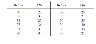
Before an increase in speed enforcement activities:
The speed ranges from 28 to 40 mi/hgiving a speed range of 12. For five classes, the range per class is 2.4mi/h. A frequency distribution table can then be prepared, as shown below, in which the speed classes are listed in column 1 and the mid-values are in column 2. The number of observationsfor each class is listed in column 3, the cumulative percentages of all observations arelisted in column 6.
| 1 | 2 | 3 | 4 | 5 | 6 | 7 |
| Speed class (mi/h) | Class mid-value | Class frequency, | | Percentage of class frequency | Cumulative percentage of class frequency | |
| 28-30 | 29 | 4 | 116 | 13 | 13 | 139.24 |
| 31-33 | 32 | 5 | 160 | 17 | 30 | 42.05 |
| 34-36 | 35 | 12 | 420 | 40 | 70 | 0.12 |
| 37-39 | 38 | 6 | 228 | 20 | 90 | 57.66 |
| 40-42 | 41 | 3 | 123 | 10 | 100 | 111.63 |
| Total | 30 | 1047 | 350.7 |
Determine the arithmetic mean speed:
Determine the standard deviation:
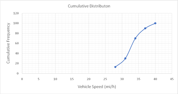
The 85th-percentile speed is obtained from the cumulative frequency distribution curve as 36 mi/h.
The percentage of traffic exceeding the posted speed limit of 30 mi/h is 76 %.
Below given figure shows the cumulative frequency distribution curve for the data given. In this case, the cumulative percentages in column 6 of the above Table are plotted against the upper limit of each corresponding speed class. This curve, therefore, gives the percentage of vehicles that are traveling at or below a given speed.
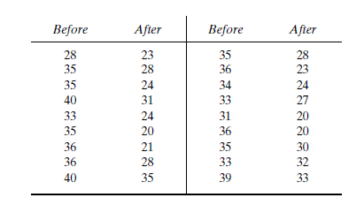
After an increase in speed enforcement activities:
The speed ranges from 20 to 37 mi/h giving a speed range of 17. For six classes, the range per class is 2.83 mi/h. A frequency distribution table can then be prepared, as shown below in which the speed classes are listed in column 1 and the mid-values are in column 2. The number of observations for each class is listed in column 3, the cumulative percentages of all observations are listed in column 6.
| 1 | 2 | 3 | 4 | 5 | 6 | 7 |
| Speed class (mi/h) | Class mid-value | Class frequency, | | Percentage of class frequency | Cumulative percentage of class frequency | |
| 20-22 | 21 | 6 | 126 | 20 | 20 | 253.5 |
| 23-25 | 24 | 8 | 192 | 27 | 47 | 98 |
| 26-28 | 27 | 4 | 108 | 13 | 60 | 1 |
| 29-31 | 30 | 3 | 90 | 10 | 70 | 18.75 |
| 32-34 | 33 | 5 | 165 | 17 | 87 | 151.25 |
| 35-37 | 36 | 4 | 144 | 13 | 100 | 289 |
| Total | 30 | 825 | 811.5 |
Determine the arithmetic mean speed:
Determine the standard deviation:
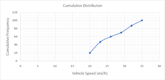
Below given figure shows the cumulative frequency distribution curve for the data given. In this case, the cumulative percentages in column 6 of the above Table are plotted against the upper limit of each corresponding speed class. This curve, therefore, gives the percentage of vehicles that are traveling at or below a given speed.
The 85th-percentile speed is obtained from the cumulative frequency distribution curve as 31.5 mi/h.
The percentage of traffic exceeding the posted speed limit of 30 mi/h is 24 %.
Determine square root of the pooled variance:
Compute test static T:
Determine whether
From Appendix A, theoretical
Since
Conclusion:
The increase in speed enforcement activities has resulted in a significant reduction in the mean speed on the street at a significance level of 0.05. The mean speeds before and after increase in speed enforcement activities are 35.1 and 27.47 mi/h respectively. The standard deviations are 3.5 and 5.3 mi/h respectively. The 85th percentile speeds are 36 mi/h and 31.5 mi/h and percentages of traffic exceeding the posted speed limit of 30 mi/h are 76 % and 24 %.
Want to see more full solutions like this?
Chapter 4 Solutions
Traffic and Highway Engineering

- quantity surveyingarrow_forwardNote: Please accurately answer it!. I'll give it a thumbs up or down based on the answer quality and precision. Question: What is the group name of Sample B in problem 3 from the image?. By also using the ASTM flow chart!. This unit is soil mechanics btwarrow_forwardPick the rural location of a project site in Victoria, and its catchment area-not bigger than 25 sqkm, and given the below information, determine the rainfall intensity for ARI = 5, 50, 100 year storm event. Show all the details of the procedure. Each student must propose different length of streams and elevations. Use fig below as a sample only. Pt. E-ht. 95.0 200m 600m PLD-M. 91.0 300m Pt. C-93.0 300m PL.B-ht. 92.0 PL.F-ht. 96.0 500m Pt. A-M. 91.00 To be deemed satisfactory the solution must include: Q.F1.1.Choice of catchment location Q.F1.2. A sketch displaying length of stream and elevation Q.F1.3. Catchment's IFD obtained from the Buro of Metheorology for specified ARI Q.F1.4.Calculation of the time of concentration-this must include a detailed determination of the equivalent slope. Q.F1.5.Use must be made of the Bransby-Williams method for the determination of the equivalent slope. Q.F1.6.The graphical display of the estimation of intensities for ARI 5,50, 100 must be shown.arrow_forward
- QUANTITY SURVEYINGarrow_forward3. (a) Use method of joints to determine forces in all members (all distances are in mm) (b) Find the resultant force at the pin support and state its angle of inclination FIGURE 2 2400 3.3 kN 6 3.6 ky 12 2 + 2400 0.7 kN + 2400 3.3kN + 2400arrow_forwardOK i need help. Please help me work thorought this with autocad. I am not sure where to begin but i need to draw this. Well if you read the question we did it in class and I got suepr confsued.arrow_forward
- A square column foundation has to carry a gross allowable load of 2005 kN (FS = 3). Given: D₤ = 1.7 m, y = 15.9 kN/m³, 0' = 34°, and c' = 0. Use Terzaghi's equation to determine the size of the foundation (B). Assume general shear failure. For o' = 34°, N₁ 36.5 and Ny = 38.04. (Enter your answer to three significant figures.) B=2.16 marrow_forwardFor the design of a shallow foundation, given the following: Soil: ' = 20° c=57 kN/m² Unit weight, y=18 kN/m³ Modulus of elasticity, E, = 1400 kN/m² Poisson's ratio, μs = 0.35 Foundation: L=2m B=1m D₁ =1m Calculate the ultimate bearing capacity. Use the equation: 1 qu= c'Ne Fes Fed Fec +qNqFqs FqdFqc + - BNF √s F√d F 2 For d'=20°, N = 14.83, N = 6.4, and N., = 5.39. (Enter your answer to three significant figures.) qu kN/m²arrow_forward1.0 m (Eccentricity in one direction only) = 0.15 m Qall = 0 1.5 m x 1.5 m Centerline An eccentrically loaded foundation is shown in the figure above. Use FS of 4 and determine the maximum allowable load that the foundation can carry if y = 16 kN/m³ and ' = 35°. Use Meyerhof's effective area method. For o' = 35°, N₁ = 33.30 and Ny = 48.03. (Enter your answer to three significant figures.) Qall kNarrow_forward
- Methyl alcohol at 25°C (ρ = 789 kg/m³, μ = 5.6 × 10⁻⁴ kg/m∙s) flows through the system below at a rate of 0.015 m³/s. Fluid enters the suction line from reservoir 1 (left) through a sharp-edged inlet. The suction line is 10 cm commercial steel pipe, 15 m long. Flow passes through a pump with efficiency of 76%. Flow is discharged from the pump into a 5 cm line, through a fully open globe valve and a standard smooth threaded 90° elbow before reaching a long, straight discharge line. The discharge line is 5 cm commercial steel pipe, 200 m long. Flow then passes a second standard smooth threaded 90° elbow before discharging through a sharp-edged exit to reservoir 2 (right). Pipe lengths between the pump and valve, and connecting the second elbow to the exit are negligibly short compared to the suction and discharge lines. Volumes of reservoirs 1 and 2 are large compared to volumes extracted or supplied by the suction and discharge lines. Calculate the power that must be supplied to the…arrow_forwardcan you help me figure out the calculations so that i can input into autocad? Not apart of a graded assinment. Just a problem in class that i missed.arrow_forwardUse method of joints to determine forces in all members (all distances are in mm) Find the resultant force at the pin support and state its angle of inclinationarrow_forward
 Traffic and Highway EngineeringCivil EngineeringISBN:9781305156241Author:Garber, Nicholas J.Publisher:Cengage Learning