Videos
a.
Arrange the data and obtain Xmin and Xmax.
a.
Answer to Problem 95CE
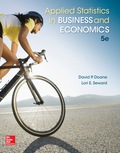
The value of Xmin is 0.9.
The value of Xmax is 11.9.
Explanation of Solution
Calculation:
The data state to choose a dataset to prepare a brief descriptive report.
Here, the data chosen is Data set A.
The Data set A represents the percentage of sales in selected industries.
The data set A of sales percent can be sorted either ascending or descending.
Here, the data is sorted in the ascending order.
Sorting:
Software procedure:
Step-by-step procedure to sort the data using the MINITAB software:
- • Choose Data > Sort.
- • In columns to sort by, enter Percent.
- • Under Columns to sort, Choose specified columns.
- • In columns, enter the percent and choose increasing option.
- • In storage location for current columns, choose “specified columns of the current worksheet”.
- • In columns, enter “sorted percent”.
- • Click ok.
Thus, the sorted data has been stored in the column of sorted percent.
Minimum and Maximum:
Step-by-step procedure to find the minimum and maximum using the MINITAB software:
- • Choose Calc>calculator.
- • In store result in variable box, enter Minimum.
- • Under Expression, enter “MIN(Percent)”.
- • Click ok.
- • Choose Calc>calculator.
- • In store result in variable box, enter Maximum.
- • Under Expression, enter “MAX(Percent)”.
- • Click ok.
Data display:
- • Choose data> display data.
- • Select the columns to display as Minimum, Maximum.
- • Click ok.
Output using the MINITAB software is given below:
Thus, the value of Xmin is 0.9 and the value of Xmax is 11.9 respectively.
b.
Construct a histogram.
b.
Answer to Problem 95CE
Histogram:
Output obtained from MINITAB software is:
Explanation of Solution
Calculation:
Software procedure:
- Step by step procedure to draw the Histogram using MINITAB software.
- • Choose Graph > Histogram.
- • Choose Simple, and then click OK.
- • In Graph variables, enter the Percent.
- • Click OK.
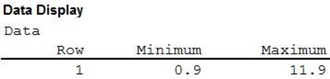
Thus, the histogram has been obtained.
By observing the graph, it is clear that the curve is right skewed. Hence, it is appropriate to conclude that the data is approximately right skewed. Thus, the data set A for percent of sales is approximately right skewed.
c.
Find the
c.
Answer to Problem 95CE
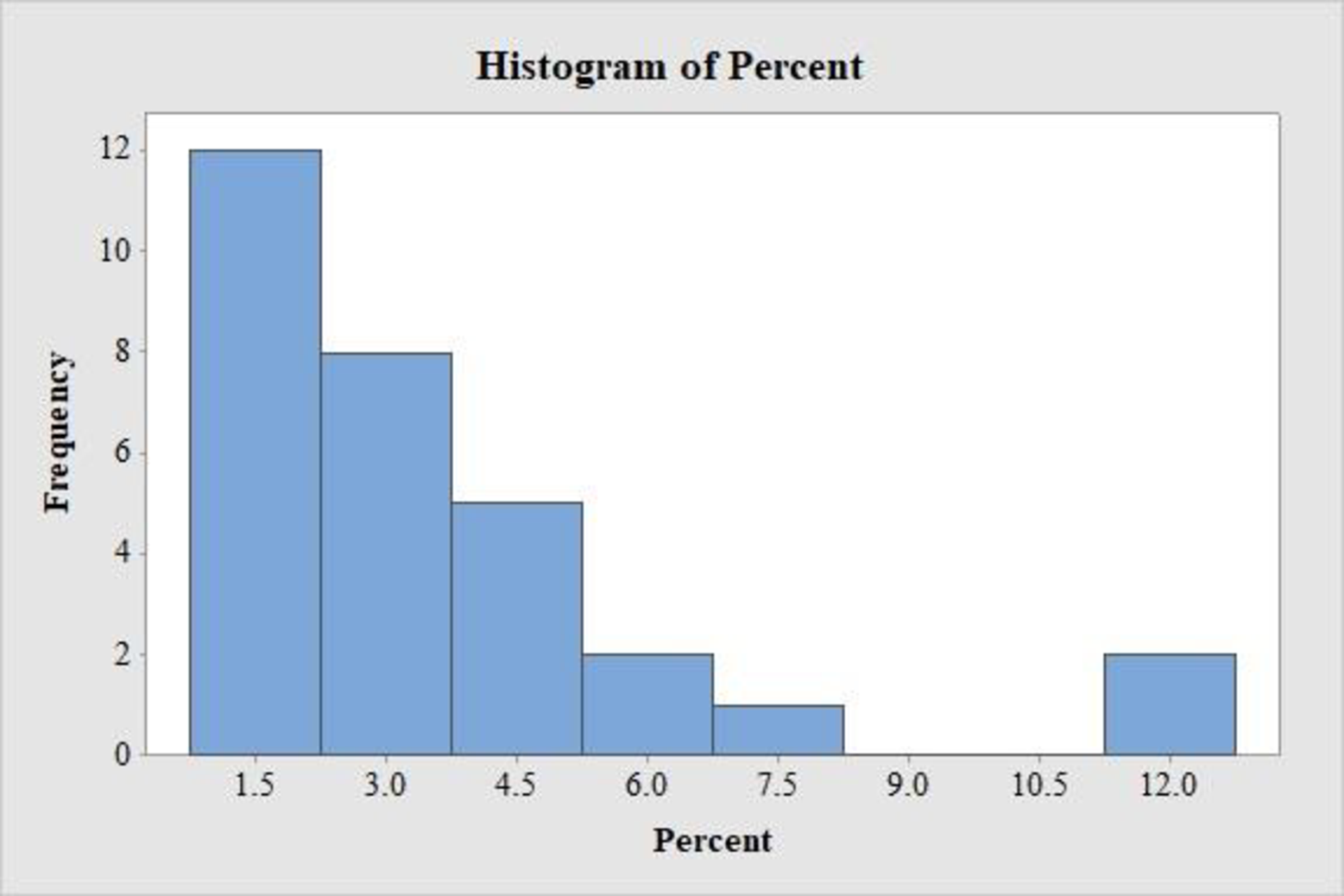
The mean score is 3.55.
The median score is 3.
Explanation of Solution
Calculation:
Mean and median:
Software procedure:
Step-by-step procedure to find the mean, the median using the MINITAB software:
- • Choose Stat > Basic Statistics > Display
Descriptive Statistics . - • In Variables enter the columns Percent.
- • Choose option statistics, and select Mean, Median.
- • Click OK.
Output using the MINITAB software is given below:
- Thus, the mean and the median for the data set A are 3.55 and 3 respectively.
Shape of the distribution:
- • For symmetric data, the mean, the median and the
mode are equal. - • For positively skewed data, the mean exceeds the median.
- • For negatively skewed data, the mean is lower than the median.
From the value of mean, median, it is observed that the value of mean is greater than that of the median.
Thus, the data is said to be right skewed or positively skewed.
d.
Find the standard deviation for data set A.
d.
Answer to Problem 95CE
The standard deviation for data set A is 2.749.
Explanation of Solution
Calculation:
Standard deviation:
Software procedure:
Step-by-step procedure to find the mean and standard deviation using the MINITAB software:
- • Choose Stat > Basic Statistics > Display Descriptive Statistics.
- • In Variables enter the columns Percent.
- • Choose option statistics, and select Standard deviation.
- • Click OK.
Output using the MINITAB software is given below:
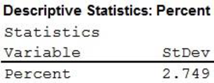
- Thus, the standard deviation has been obtained.
f.
Standardize the data and identify the outliers and an unusual observations.
f.
Answer to Problem 95CE
The standardized values of dataset A are given below:
| -0.9640 | -0.6366 | 0.3456 | 0.3820 | -0.6730 | 0.0909 |
| 0.7093 | -0.0182 | -0.0182 | -0.9276 | -0.1637 | -0.2001 |
| 1.4005 | -0.9640 | -0.8912 | -0.0182 | 3.0375 | -0.6002 |
| -0.8185 | 1.0367 | -0.2001 | -0.4547 | 0.2728 | -0.6366 |
| -0.8912 | -0.5638 | -0.5638 | 0.4911 | -0.3820 | 2.8192 |
There are two outliers and two unusual values in the dataset.
Explanation of Solution
Calculation:
Standardized values:
Software procedure:
Step-by-step software procedure to obtain standardized values using EXCEL software is as follows:
- • Open an EXCEL file.
- • Enter the data in the column A in cells A1 to A32.
- • In cell B1, enter the formula “=STANDARDIZE(A1, 3.55, 2.749)”.
- • Select “ENTER” option.
- • Select and copy the cell B1 and drag till the 30nd cell.
- Output using EXCEL software is given below:
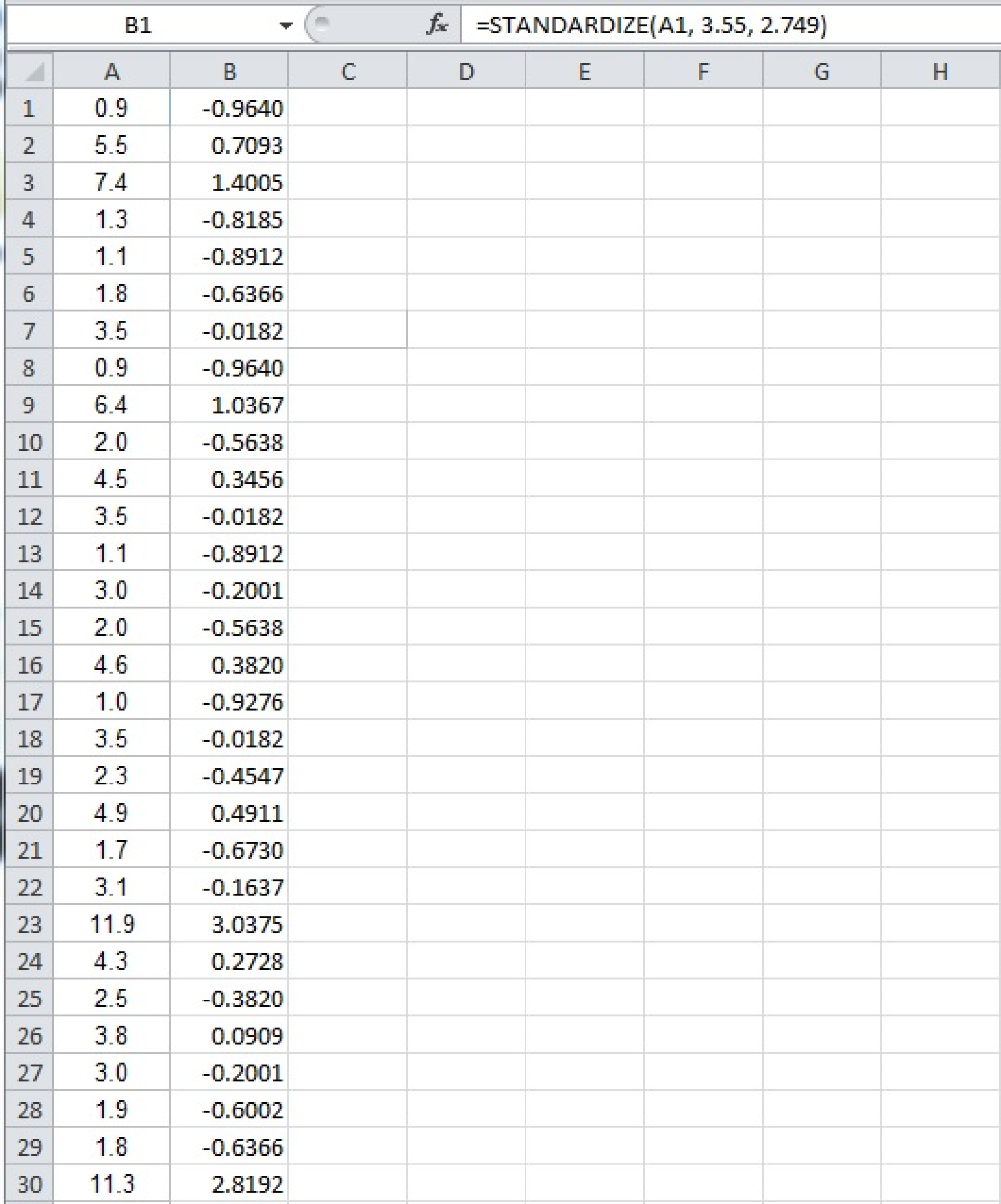
Thus, the standardized values have been obtained using EXCEL.
The outliers in the data set A can be identified using
Empirical Rule:
The Empirical Rule for a Normal model states that:
- • Within 1 standard deviation of mean, 68.26% of all observations will lie.
- • Within 2 standard deviations of mean, 95.44% of all observations will lie.
- • Within 3 standard deviations of mean, 99.73% of all observations will lie.
Empirical rule using MEGASTAT:
Software procedure:
Step-by-step software procedure to obtain Empirical rule using Mega Stat software is as follows:
- • Open an EXCEL file.
- • Enter the data in the column A in cells A1 to A30.
- • From the Add-Ins, Select Mega Stat >Descriptive statistics.
- • A dialogue box appears.
- • In Input
range box, select the input range from Sheet1!$A$1:$A$30. - • From the list box, select Empirical rule.
- • Click “OK”.
Output obtained using MEGA STAT is as follows:
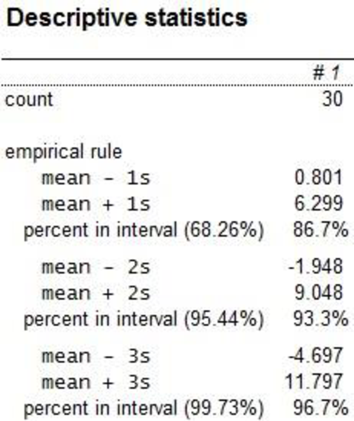
The upper and lower bounds for the intervals indicated by the Empirical rule have been obtained.
Based on the z-scores, the observation has one outlier, that is, the observations with values 11.9 do not lie within the 3-standard deviations limits (–4.697 to 11.797). there is no unusual observation in the data set A.
f.
Find the
f.
Answer to Problem 95CE
The Q1 (25th percentile) is 1.775, Q2 (50th percentile) is 3 and Q3 (75th percentile) is 4.525.
Explanation of Solution
Calculation:
Standard deviation:
Software procedure:
Step-by-step procedure to find the Quartiles using the MINITAB software:
- • Choose Stat > Basic Statistics > Display Descriptive Statistics.
- • In Variables enter the columns Percent.
- • Choose option statistics, and select First Quartile, Median and Third Quartile.
- • Choose option Graphs, and select boxplot of data.
- • Click OK.
Output using the MINITAB software is given below:
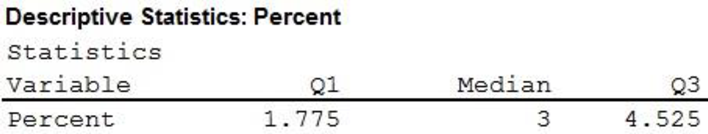
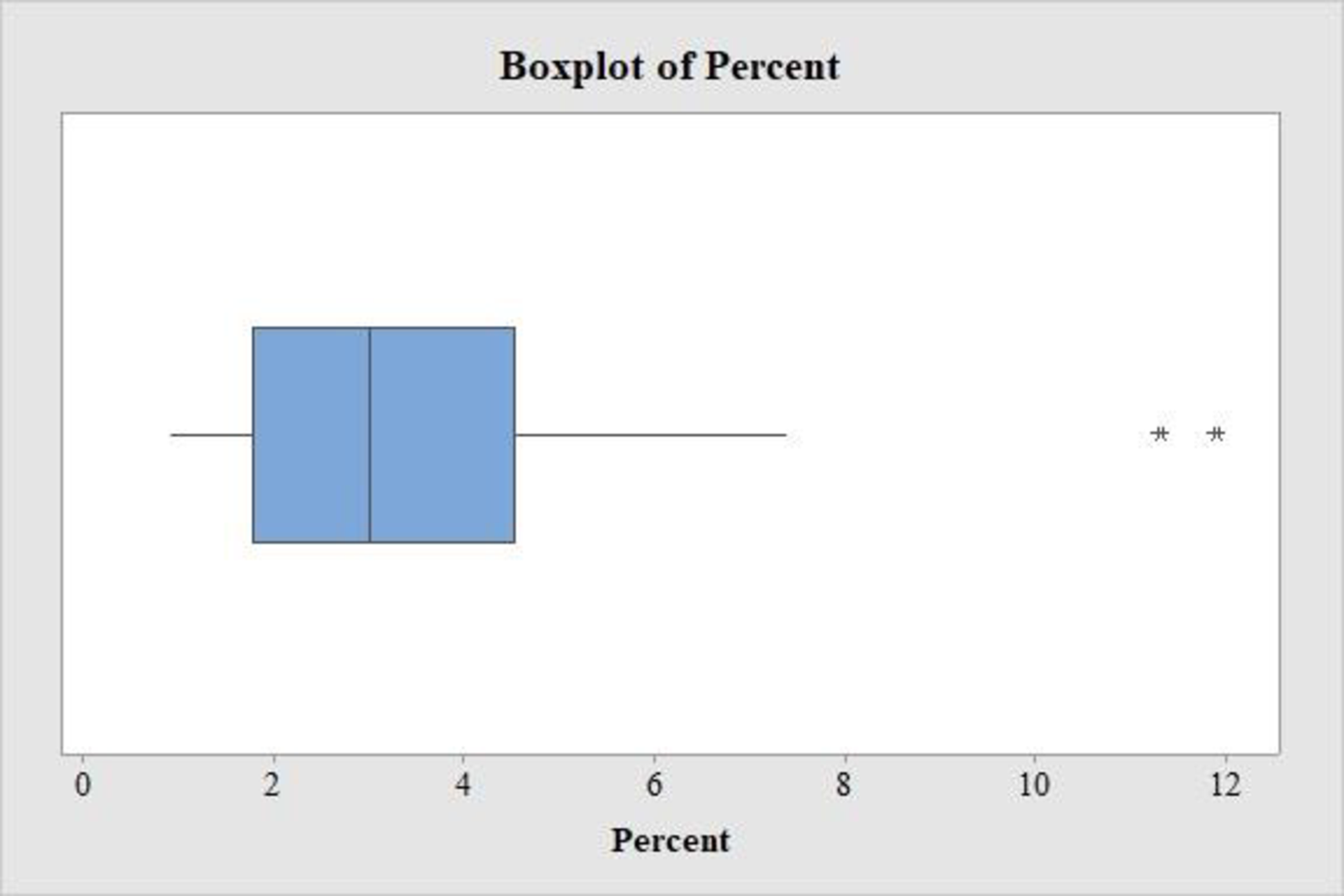
- Thus, the Quartiles and boxplot have been obtained.
Observation:
From the boxplot, it is observed that the data set has two outliers within it. The boxplot disclosed that the median is closer to the first quartile, Q1 than it is to the third quartile, Q3, suggesting that the data is right skewed. The whiskers on the two sides are close in length, although it appears that the left whisker is slightly longer.
Want to see more full solutions like this?
Chapter 4 Solutions
Applied Statistics in Business and Economics


- II Consider the following data matrix X: X1 X2 0.5 0.4 0.2 0.5 0.5 0.5 10.3 10 10.1 10.4 10.1 10.5 What will the resulting clusters be when using the k-Means method with k = 2. In your own words, explain why this result is indeed expected, i.e. why this clustering minimises the ESS map.arrow_forwardwhy the answer is 3 and 10?arrow_forwardPS 9 Two films are shown on screen A and screen B at a cinema each evening. The numbers of people viewing the films on 12 consecutive evenings are shown in the back-to-back stem-and-leaf diagram. Screen A (12) Screen B (12) 8 037 34 7 6 4 0 534 74 1645678 92 71689 Key: 116|4 represents 61 viewers for A and 64 viewers for B A second stem-and-leaf diagram (with rows of the same width as the previous diagram) is drawn showing the total number of people viewing films at the cinema on each of these 12 evenings. Find the least and greatest possible number of rows that this second diagram could have. TIP On the evening when 30 people viewed films on screen A, there could have been as few as 37 or as many as 79 people viewing films on screen B.arrow_forward
- Q.2.4 There are twelve (12) teams participating in a pub quiz. What is the probability of correctly predicting the top three teams at the end of the competition, in the correct order? Give your final answer as a fraction in its simplest form.arrow_forwardThe table below indicates the number of years of experience of a sample of employees who work on a particular production line and the corresponding number of units of a good that each employee produced last month. Years of Experience (x) Number of Goods (y) 11 63 5 57 1 48 4 54 5 45 3 51 Q.1.1 By completing the table below and then applying the relevant formulae, determine the line of best fit for this bivariate data set. Do NOT change the units for the variables. X y X2 xy Ex= Ey= EX2 EXY= Q.1.2 Estimate the number of units of the good that would have been produced last month by an employee with 8 years of experience. Q.1.3 Using your calculator, determine the coefficient of correlation for the data set. Interpret your answer. Q.1.4 Compute the coefficient of determination for the data set. Interpret your answer.arrow_forwardCan you answer this question for mearrow_forward
- Techniques QUAT6221 2025 PT B... TM Tabudi Maphoru Activities Assessments Class Progress lIE Library • Help v The table below shows the prices (R) and quantities (kg) of rice, meat and potatoes items bought during 2013 and 2014: 2013 2014 P1Qo PoQo Q1Po P1Q1 Price Ро Quantity Qo Price P1 Quantity Q1 Rice 7 80 6 70 480 560 490 420 Meat 30 50 35 60 1 750 1 500 1 800 2 100 Potatoes 3 100 3 100 300 300 300 300 TOTAL 40 230 44 230 2 530 2 360 2 590 2 820 Instructions: 1 Corall dawn to tha bottom of thir ceraan urina se se tha haca nariad in archerca antarand cubmit Q Search ENG US 口X 2025/05arrow_forwardThe table below indicates the number of years of experience of a sample of employees who work on a particular production line and the corresponding number of units of a good that each employee produced last month. Years of Experience (x) Number of Goods (y) 11 63 5 57 1 48 4 54 45 3 51 Q.1.1 By completing the table below and then applying the relevant formulae, determine the line of best fit for this bivariate data set. Do NOT change the units for the variables. X y X2 xy Ex= Ey= EX2 EXY= Q.1.2 Estimate the number of units of the good that would have been produced last month by an employee with 8 years of experience. Q.1.3 Using your calculator, determine the coefficient of correlation for the data set. Interpret your answer. Q.1.4 Compute the coefficient of determination for the data set. Interpret your answer.arrow_forwardQ.3.2 A sample of consumers was asked to name their favourite fruit. The results regarding the popularity of the different fruits are given in the following table. Type of Fruit Number of Consumers Banana 25 Apple 20 Orange 5 TOTAL 50 Draw a bar chart to graphically illustrate the results given in the table.arrow_forward
- Q.2.3 The probability that a randomly selected employee of Company Z is female is 0.75. The probability that an employee of the same company works in the Production department, given that the employee is female, is 0.25. What is the probability that a randomly selected employee of the company will be female and will work in the Production department? Q.2.4 There are twelve (12) teams participating in a pub quiz. What is the probability of correctly predicting the top three teams at the end of the competition, in the correct order? Give your final answer as a fraction in its simplest form.arrow_forwardQ.2.1 A bag contains 13 red and 9 green marbles. You are asked to select two (2) marbles from the bag. The first marble selected will not be placed back into the bag. Q.2.1.1 Construct a probability tree to indicate the various possible outcomes and their probabilities (as fractions). Q.2.1.2 What is the probability that the two selected marbles will be the same colour? Q.2.2 The following contingency table gives the results of a sample survey of South African male and female respondents with regard to their preferred brand of sports watch: PREFERRED BRAND OF SPORTS WATCH Samsung Apple Garmin TOTAL No. of Females 30 100 40 170 No. of Males 75 125 80 280 TOTAL 105 225 120 450 Q.2.2.1 What is the probability of randomly selecting a respondent from the sample who prefers Garmin? Q.2.2.2 What is the probability of randomly selecting a respondent from the sample who is not female? Q.2.2.3 What is the probability of randomly…arrow_forwardTest the claim that a student's pulse rate is different when taking a quiz than attending a regular class. The mean pulse rate difference is 2.7 with 10 students. Use a significance level of 0.005. Pulse rate difference(Quiz - Lecture) 2 -1 5 -8 1 20 15 -4 9 -12arrow_forward
 MATLAB: An Introduction with ApplicationsStatisticsISBN:9781119256830Author:Amos GilatPublisher:John Wiley & Sons Inc
 Probability and Statistics for Engineering and th...StatisticsISBN:9781305251809Author:Jay L. DevorePublisher:Cengage Learning
 Statistics for The Behavioral Sciences (MindTap C...StatisticsISBN:9781305504912Author:Frederick J Gravetter, Larry B. WallnauPublisher:Cengage Learning
 Elementary Statistics: Picturing the World (7th E...StatisticsISBN:9780134683416Author:Ron Larson, Betsy FarberPublisher:PEARSON
 The Basic Practice of StatisticsStatisticsISBN:9781319042578Author:David S. Moore, William I. Notz, Michael A. FlignerPublisher:W. H. Freeman
 Introduction to the Practice of StatisticsStatisticsISBN:9781319013387Author:David S. Moore, George P. McCabe, Bruce A. CraigPublisher:W. H. Freeman