Concept explainers
Videos
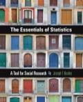
Median Income for Canadian Provinces and Territories, 2000 and 2011 (Canadian dollars)
| Province or Territory | 2000 | 2011 |
| Newfoundland and Labrador | 38,800 | 67,200 |
| Prince Edward Island | 44,200 | 66,500 |
| Nova Scotia | 44,500 | 66,300 |
| New Brunswick | 43,200 | 63,930 |
| Quebec | 47,700 | 68,170 |
| Ontario | 55,700 | 73,290 |
| Manitoba | 47,300 | 68,710 |
| Saskatchewan | 45,800 | 77,300 |
| Alberta | 55,200 | 89,930 |
| British Columbia | 49,100 | 69,150 |
| Yukon Columbia | 56,000 | 90,090 |
| Northwest Territories | 61,000 | 105,560 |
| Nunavut | 37,600 | 65,280 |
|
|
||
|
|
||
|
|
||
|
|
Median Income for Thirteen States, 1999 and 2012 (U.S dollars)
| State | 1999 | 2012 |
| Alabama | 36,213 | 43,464 |
| Alaska | 51,509 | 63,348 |
| Arkansas | 29,762 | 39,018 |
| California | 43,744 | 57,020 |
| Connecticut | 50,798 | 64,247 |
| Illinois | 46,392 | 51,738 |
| Kansas | 37,476 | 50,003 |
| Maryland | 52,310 | 71,836 |
| Michigan | 46,238 | 50,015 |
| New York | 40,058 | 47,680 |
| Ohio | 39,617 | 44,375 |
| South Dakota | 35,962 | 49,415 |
| Texas | 38,978 | 51,926 |
|
|
||
|
|
||
|
|
||
|
|
3.6
Median Income for Canadian Provinces and Territories, 2000 and 2011 (Canadian dollars)
| Province or Territory | 2000 | 2011 |
| Newfoundland and Labrador | 38,800 | 67,200 |
| Prince Edward Island | 44,200 | 66,500 |
| Nova Scotia | 44,500 | 66,300 |
| New Brunswick | 43,200 | 63,930 |
| Quebec | 47,700 | 68,170 |
| Ontario | 55,700 | 73,290 |
| Manitoba | 47,300 | 68,710 |
| Saskatchewan | 45,800 | 77,300 |
| Alberta | 55,200 | 89,930 |
| British Columbia | 49,100 | 69,150 |
| Yukon Columbia | 56,000 | 90,090 |
| Northwest Territories | 61,000 | 105,560 |
| Nunavut | 37,600 | 65,280 |
|
|
||
|
|
Median Income for Thirteen States, 1999 and 2012 (U.S dollars)
| State | 1999 | 2012 |
| Alabama | 36,213 | 43,464 |
| Alaska | 51,509 | 63,348 |
| Arkansas | 29,762 | 39,018 |
| California | 43,744 | 57,020 |
| Connecticut | 50,798 | 64,247 |
| Illinois | 46,392 | 51,738 |
| Kansas | 37,476 | 50,003 |
| Maryland | 52,310 | 71,836 |
| Michigan | 46,238 | 50,015 |
| New York | 40,058 | 47,680 |
| Ohio | 39,617 | 44,375 |
| South Dakota | 35,962 | 49,415 |
| Texas | 38,978 | 51,926 |
|
|
||
|
|
Want to see the full answer?
Check out a sample textbook solution
Chapter 4 Solutions
Essentials Of Statistics
Additional Math Textbook Solutions
Elementary & Intermediate Algebra
Intermediate Algebra (13th Edition)
Elementary Statistics: Picturing the World (7th Edition)
Elementary Statistics ( 3rd International Edition ) Isbn:9781260092561
Finite Mathematics for Business, Economics, Life Sciences and Social Sciences


- An electronics company manufactures batches of n circuit boards. Before a batch is approved for shipment, m boards are randomly selected from the batch and tested. The batch is rejected if more than d boards in the sample are found to be faulty. a) A batch actually contains six faulty circuit boards. Find the probability that the batch is rejected when n = 20, m = 5, and d = 1. b) A batch actually contains nine faulty circuit boards. Find the probability that the batch is rejected when n = 30, m = 10, and d = 1.arrow_forwardTwenty-eight applicants interested in working for the Food Stamp program took an examination designed to measure their aptitude for social work. A stem-and-leaf plot of the 28 scores appears below, where the first column is the count per branch, the second column is the stem value, and the remaining digits are the leaves. a) List all the values. Count 1 Stems Leaves 4 6 1 4 6 567 9 3688 026799 9 8 145667788 7 9 1234788 b) Calculate the first quartile (Q1) and the third Quartile (Q3). c) Calculate the interquartile range. d) Construct a boxplot for this data.arrow_forwardPam, Rob and Sam get a cake that is one-third chocolate, one-third vanilla, and one-third strawberry as shown below. They wish to fairly divide the cake using the lone chooser method. Pam likes strawberry twice as much as chocolate or vanilla. Rob only likes chocolate. Sam, the chooser, likes vanilla and strawberry twice as much as chocolate. In the first division, Pam cuts the strawberry piece off and lets Rob choose his favorite piece. Based on that, Rob chooses the chocolate and vanilla parts. Note: All cuts made to the cake shown below are vertical.Which is a second division that Rob would make of his share of the cake?arrow_forward
- Three players (one divider and two choosers) are going to divide a cake fairly using the lone divider method. The divider cuts the cake into three slices (s1, s2, and s3). If the choosers' declarations are Chooser 1: {s1 , s2} and Chooser 2: {s2 , s3}. Using the lone-divider method, how many different fair divisions of this cake are possible?arrow_forwardTheorem 2.6 (The Minkowski inequality) Let p≥1. Suppose that X and Y are random variables, such that E|X|P <∞ and E|Y P <00. Then X+YpX+Yparrow_forwardTheorem 1.2 (1) Suppose that P(|X|≤b) = 1 for some b > 0, that EX = 0, and set Var X = 0². Then, for 0 0, P(X > x) ≤e-x+1²² P(|X|>x) ≤2e-1x+1²² (ii) Let X1, X2...., Xn be independent random variables with mean 0, suppose that P(X ≤b) = 1 for all k, and set oσ = Var X. Then, for x > 0. and 0x) ≤2 exp Σ k=1 (iii) If, in addition, X1, X2, X, are identically distributed, then P(S|x) ≤2 expl-tx+nt²o).arrow_forward
- Theorem 5.1 (Jensen's inequality) state without proof the Jensen's Ineg. Let X be a random variable, g a convex function, and suppose that X and g(X) are integrable. Then g(EX) < Eg(X).arrow_forwardCan social media mistakes hurt your chances of finding a job? According to a survey of 1,000 hiring managers across many different industries, 76% claim that they use social media sites to research prospective candidates for any job. Calculate the probabilities of the following events. (Round your answers to three decimal places.) answer parts a-c. a) Out of 30 job listings, at least 19 will conduct social media screening. b) Out of 30 job listings, fewer than 17 will conduct social media screening. c) Out of 30 job listings, exactly between 19 and 22 (including 19 and 22) will conduct social media screening. show all steps for probabilities please. answer parts a-c.arrow_forwardQuestion: we know that for rt. (x+ys s ا. 13. rs. and my so using this, show that it vye and EIXI, EIYO This : E (IX + Y) ≤2" (EIX (" + Ely!")arrow_forward
- Theorem 2.4 (The Hölder inequality) Let p+q=1. If E|X|P < ∞ and E|Y| < ∞, then . |EXY ≤ E|XY|||X|| ||||qarrow_forwardTheorem 7.6 (Etemadi's inequality) Let X1, X2, X, be independent random variables. Then, for all x > 0, P(max |S|>3x) ≤3 max P(S| > x). Isk≤narrow_forwardTheorem 7.2 Suppose that E X = 0 for all k, that Var X = 0} x) ≤ 2P(S>x 1≤k≤n S√2), -S√2). P(max Sk>x) ≤ 2P(|S|>x- 1arrow_forwardarrow_back_iosSEE MORE QUESTIONSarrow_forward_ios
 Glencoe Algebra 1, Student Edition, 9780079039897...AlgebraISBN:9780079039897Author:CarterPublisher:McGraw Hill