Concept explainers
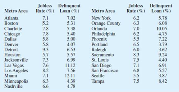
At the beginning of 2009, the economic downturn resulted in the loss of jobs and an increase in delinquent loans for housing. The national unemployment rate was 6.5% and the percentage of delinquent loans was 6.12% (The Wall Street Journal, January 27, 2009). In projecting where the real estate market was headed in the coming year, economists studied the relationship between the jobless rate and the percentage of delinquent loans. The expectation was that if the jobless rate continued to increase, there would also be an

increase in the percentage of delinquent loans. The data below show the jobless rate and the delinquent loan percentage for 27 major real estate markets.
- a. Compute the
correlation coefficient . Is there apositive correlation between the jobless rate and the percentage of delinquent housing loans? What is your interpretation? - b. Show a
scatter diagram of the relationship between jobless rate and the percentage of delinquent housing loans.
Trending nowThis is a popular solution!

Chapter 3 Solutions
Statistics for Business & Economics, Revised (MindTap Course List)
- 1.2.17. (!) Let G,, be the graph whose vertices are the permutations of (1,..., n}, with two permutations a₁, ..., a,, and b₁, ..., b, adjacent if they differ by interchanging a pair of adjacent entries (G3 shown below). Prove that G,, is connected. 132 123 213 312 321 231arrow_forwardYou are planning an experiment to determine the effect of the brand of gasoline and the weight of a car on gas mileage measured in miles per gallon. You will use a single test car, adding weights so that its total weight is 3000, 3500, or 4000 pounds. The car will drive on a test track at each weight using each of Amoco, Marathon, and Speedway gasoline. Which is the best way to organize the study? Start with 3000 pounds and Amoco and run the car on the test track. Then do 3500 and 4000 pounds. Change to Marathon and go through the three weights in order. Then change to Speedway and do the three weights in order once more. Start with 3000 pounds and Amoco and run the car on the test track. Then change to Marathon and then to Speedway without changing the weight. Then add weights to get 3500 pounds and go through the three gasolines in the same order.Then change to 4000 pounds and do the three gasolines in order again. Choose a gasoline at random, and run the car with this gasoline at…arrow_forwardAP1.2 A child is 40 inches tall, which places her at the 90th percentile of all children of similar age. The heights for children of this age form an approximately Normal distribution with a mean of 38 inches. Based on this information, what is the standard deviation of the heights of all children of this age? 0.20 inches (c) 0.65 inches (e) 1.56 inches 0.31 inches (d) 1.21 inchesarrow_forward
- AP1.1 You look at real estate ads for houses in Sarasota, Florida. Many houses range from $200,000 to $400,000 in price. The few houses on the water, however, have prices up to $15 million. Which of the following statements best describes the distribution of home prices in Sarasota? The distribution is most likely skewed to the left, and the mean is greater than the median. The distribution is most likely skewed to the left, and the mean is less than the median. The distribution is roughly symmetric with a few high outliers, and the mean is approximately equal to the median. The distribution is most likely skewed to the right, and the mean is greater than the median. The distribution is most likely skewed to the right, and the mean is less than the median.arrow_forwardDuring busy political seasons, many opinion polls are conducted. In apresidential race, how do you think the participants in polls are generally selected?Discuss any issues regarding simple random, stratified, systematic, cluster, andconvenience sampling in these polls. What about other types of polls, besides political?arrow_forwardPlease could you explain why 0.5 was added to each upper limpit of the intervals.Thanksarrow_forward
- 28. (a) Under what conditions do we say that two random variables X and Y are independent? (b) Demonstrate that if X and Y are independent, then it follows that E(XY) = E(X)E(Y); (e) Show by a counter example that the converse of (ii) is not necessarily true.arrow_forward1. Let X and Y be random variables and suppose that A = F. Prove that Z XI(A)+YI(A) is a random variable.arrow_forward30. (a) What is meant by the term "product measur"? ANDarrow_forward


 Trigonometry (MindTap Course List)TrigonometryISBN:9781337278461Author:Ron LarsonPublisher:Cengage Learning


