Statistics, Books a la Carte Edition Plus MyLab Statistics with Pearson eText -- Access Card Package (4th Edition)
4th Edition
ISBN: 9780134435855
Author: Alan Agresti, Christine A. Franklin, Bernhard Klingenberg
Publisher: PEARSON
expand_more
expand_more
format_list_bulleted
Concept explainers
Videos
Textbook Question
Chapter 3.4, Problem 45PB
Men’s Olympic long jumps The Olympic winning men’s long jump distances (in meters) from 1896 to 2012 and the fitted regression line for predicting them using x = year are displayed in the graph below (data on website).
- a. Identify an observation that may influence the fit of the regression line. Why did you identify this observation?
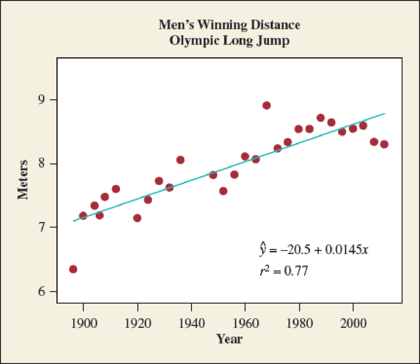
- b. Which do you think is a better prediction for the year 2016—the sample
mean of the y values in this plot or the value obtained by plugging 2016 into the fitted regression equation? - c. Would you feel comfortable using the regression line shown to predict the winning long jump for men in the year 2100? Why or why not?
Expert Solution & Answer
Want to see the full answer?
Check out a sample textbook solution
Students have asked these similar questions
C4 Q6 V1: Randomly collected student data in the dataset STATISTICSSTUDENTSSURVEYFORR contains the columns FEDBEST (preferred Federal party (Conservative, Green, Liberals, or NDP) ) , UNDERGORGRAD (degree being sought (GraduateProfessional, Undergraduate) ) and GENDERIDENTITY (Female or Male or Other). Make a crosstab (contingency) table of the counts for each of the (UNDERGORGRAD, FEDBEST) pairs for ONLY the females. If we randomly select a female student who is pursuing a graduateprofessional degree, what is the probability that she prefers the Federal Liberals. Choose the most correct (closest) answer below.
Question 6 Answer
a.
0.128
b.
0.263
c.
0.744
d.
0.333
Install RStudio: Begin by installing RStudio on your computer. If you haven't done so, please refer to the official RStudio website for download and installation instructions.
Watch the Tutorial Video: Watch the provided video tutorial that explains how to run RStudio. Pay close attention to the steps for opening and managing data files. https://www.youtube.com/watch?v=RhJp6vSZ7z0
Open RStudio: Once RStudio is installed, open the application.
Load the Dataset: In RStudio, open a data file named "mtcars". To do this, type the command mtcars in the script editor and run the command.
Attach the Data: Next, attach the dataset using the command attach(mtcars).
Examine the Variables: Carefully review and note the names of all variables in the dataset. Examples of these variables include:
Mileage (mpg)
Number of Cylinders (cyl)
Displacement (disp)
Horsepower (hp)
Research: Google to understand these variables.
Statistical Analysis: Select mpg variable, and perform the following…
A marketing professor has surveyed the students at her university to better understand attitudes towards PPT usage for higher education. To be able to make inferences to the entire student body, the sample drawn needs to represent the university’s student population on all key characteristics. The table below shows the five key student demographic variables. The professor found the breakdown of the overall student body in the university’s fact book posted online.
A non-parametric chi-square test was used to test the sample demographics against the population percentages shown in the table above. Review the output for the five chi-square tests on the following pages and answer the five questions:
Based on the chi-square test, which sample variables adequately represent the university’s student population and which ones do not? Support your answer by providing the p-value of the chi-square test and explaining what it means.
Using the results from Question 1, make recommendation for…
Chapter 3 Solutions
Statistics, Books a la Carte Edition Plus MyLab Statistics with Pearson eText -- Access Card Package (4th Edition)
Ch. 3.1 - Which is the response/explanatory variable? For...Ch. 3.1 - Sales and advertising Each month, the owner of...Ch. 3.1 - Does higher income make you happy? Every General...Ch. 3.1 - Diamonds The clarity and cut of a diamond are two...Ch. 3.1 - Alcohol and college students The Harvard School of...Ch. 3.1 - How to fight terrorism? A survey of 1000 adult...Ch. 3.1 - Heaven and hell Two questions on the General...Ch. 3.1 - Prob. 8PBCh. 3.1 - Gender gap in party ID In recent election years,...Ch. 3.1 - Use the GSS Go to the GSS website...
Ch. 3.2 - Used cars and direction of association For the 100...Ch. 3.2 - Broadband and GDP The Internet Use data file on...Ch. 3.2 - Prob. 13PBCh. 3.2 - Politics and newspaper reading For the FL Student...Ch. 3.2 - Prob. 15PBCh. 3.2 - Match the scatterplot with r Match the following...Ch. 3.2 - Prob. 17PBCh. 3.2 - Prob. 18PBCh. 3.2 - Prob. 19PBCh. 3.2 - Prob. 20PBCh. 3.2 - Prob. 21PBCh. 3.2 - Prob. 22PBCh. 3.2 - Prob. 23PBCh. 3.3 - Sketch plots of lines Identify the values of the...Ch. 3.3 - Prob. 25PBCh. 3.3 - Home selling prices The House Selling Prices FL...Ch. 3.3 - Prob. 27PBCh. 3.3 - Prob. 28PBCh. 3.3 - Prob. 29PBCh. 3.3 - Broadband subscribers and population The Internet...Ch. 3.3 - Prob. 31PBCh. 3.3 - Prob. 32PBCh. 3.3 - Regression between cereal sodium and sugar The...Ch. 3.3 - Prob. 34PBCh. 3.3 - Advertising and sales Each month, the owner of...Ch. 3.3 - Midtermfinal correlation For students who take...Ch. 3.3 - Predict final exam from midterm In an introductory...Ch. 3.3 - NL baseball Example 9 related y = team scoring...Ch. 3.3 - Study time and college GPA A graduate teaching...Ch. 3.3 - Oil and GDP An article in the September 16, 2006,...Ch. 3.3 - Mountain bikes revisited Is there a relationship...Ch. 3.3 - Mountain bike and suspension type Refer to the...Ch. 3.3 - Fuel Consumption Most cars are fuel efficient when...Ch. 3.4 - Extrapolating murder The SPSS figure shows the...Ch. 3.4 - Mens Olympic long jumps The Olympic winning mens...Ch. 3.4 - U.S. average annual temperatures Use the U.S....Ch. 3.4 - Murder and education Example 13 found the...Ch. 3.4 - Murder and poverty For Table 3.6, the regression...Ch. 3.4 - TV watching and the birth rate The figure shows...Ch. 3.4 - Looking for outliers Using software, analyze the...Ch. 3.4 - Regression between cereal sodium and sugar Let x =...Ch. 3.4 - Gestational period and life expectancy Does the...Ch. 3.4 - Antidrug campaigns An Associated Press story (June...Ch. 3.4 - Whats wrong with regression? Explain whats wrong...Ch. 3.4 - Education causes crime? The table shows a small...Ch. 3.4 - Death penalty and race The table shows results of...Ch. 3.4 - NAEP scores Eighth-grade math scores on the...Ch. 3.4 - Age a confounder? A study observes that the...Ch. 3 - Choose explanatory and response For the following...Ch. 3 - Graphing data For each case in the previous...Ch. 3 - Life after death for males and females In a recent...Ch. 3 - God and happiness Go to the GSS website...Ch. 3 - Degrees and income The mean annual salaries earned...Ch. 3 - Bacteria in ground turkey Consumer Reports...Ch. 3 - Women managers in the work force The following...Ch. 3 - RateMyProfessor.com The website RateMyProfessors....Ch. 3 - Women in government and economic life The OECD...Ch. 3 - African droughts and dust Is there a relationship...Ch. 3 - Crime rate and urbanization For the data in...Ch. 3 - Gestational period and life expectancy revisited...Ch. 3 - Height and paycheck The headline of an article in...Ch. 3 - Predicting college GPA An admissions officer...Ch. 3 - College GPA = high school GPA Refer to the...Ch. 3 - Whats a college degree worth? In 2002, a census...Ch. 3 - Care Weight and gas hogs: The table shows a short...Ch. 3 - Predicting Internet use from cell phone use We now...Ch. 3 - Income depends on education? For a study of...Ch. 3 - Fertility and GDP Refer to the Human Development...Ch. 3 - Women working and birth rate Using data from...Ch. 3 - Education and income The regression equation for a...Ch. 3 - Income in euros Refer to the previous exercise....Ch. 3 - Changing units for cereal data Refer to the Cereal...Ch. 3 - Murder and single-parent families For Table 3.6 on...Ch. 3 - Violent crime and college education For the U.S....Ch. 3 - Violent crime and high school education Repeat the...Ch. 3 - Crime and urbanization For the U.S. Statewide...Ch. 3 - High school graduation rates and health insurance...Ch. 3 - Womens Olympic high jumps Example 11 discussed how...Ch. 3 - Income and height A survey of adults revealed a...Ch. 3 - More TV watching goes with fewer babies? For...Ch. 3 - More sleep causes death? An Associated Press story...Ch. 3 - Ask Marilyn Marilyn vos Savant writes a column for...Ch. 3 - Time studying and GPA Is there a relationship...Ch. 3 - Warming in Newnan, Georgia Access the Newnan GA...Ch. 3 - Fluoride and AIDS An Associated Press story...Ch. 3 - Fish fights Alzheimers An AP story (July 22, 2003)...Ch. 3 - Dogs make you healthier A study published in the...Ch. 3 - Multiple choice: Correlate GPA and GRE In a study...Ch. 3 - Multiple choice: Properties of r Which of the...Ch. 3 - Multiple choice: Interpreting r One can interpret...Ch. 3 - Multiple choice: Correct statement about r Which...Ch. 3 - Multiple choice: Describing association between...Ch. 3 - Multiple choice: Slope and correlation The slope...Ch. 3 - Multiple choice: Interpretation of r2 An r2...Ch. 3 - True or false The variables y = annual income...Ch. 3 - Correlation doesnt depend on units Suppose you...Ch. 3 - When correlation = slope Consider the formula...Ch. 3 - Center of the data Consider the formula a=ybx for...Ch. 3 - Final exam regresses toward mean of midterm Let y...Ch. 3 - Activity: Guess the correlation The Guess the...
Knowledge Booster


Learn more about
Need a deep-dive on the concept behind this application? Look no further. Learn more about this topic, statistics and related others by exploring similar questions and additional content below.Similar questions
- A marketing professor has surveyed the students at her university to better understand attitudes towards PPT usage for higher education. To be able to make inferences to the entire student body, the sample drawn needs to represent the university’s student population on all key characteristics. The table below shows the five key student demographic variables. The professor found the breakdown of the overall student body in the university’s fact book posted online. A non-parametric chi-square test was used to test the sample demographics against the population percentages shown in the table above. Review the output for the five chi-square tests on the following pages and answer the five questions: Based on the chi-square test, which sample variables adequately represent the university’s student population and which ones do not? Support your answer by providing the p-value of the chi-square test and explaining what it means. Using the results from Question 1, make recommendation for…arrow_forwardA retail chain is interested in determining whether a digital video point-of-purchase (POP) display would stimulate higher sales for a brand advertised compared to the standard cardboard point-of-purchase display. To test this, a one-shot static group design experiment was conducted over a four-week period in 100 different stores. Fifty stores were randomly assigned to the control treatment (standard display) and the other 50 stores were randomly assigned to the experimental treatment (digital display). Compare the sales of the control group (standard POP) to the experimental group (digital POP). What were the average sales for the standard POP display (control group)? What were the sales for the digital display (experimental group)? What is the (mean) difference in sales between the experimental group and control group? List the null hypothesis being tested. Do you reject or retain the null hypothesis based on the results of the independent t-test? Was the difference between the…arrow_forwardWhat were the average sales for the four weeks prior to the experiment? What were the sales during the four weeks when the stores used the digital display? What is the mean difference in sales between the experimental and regular POP time periods? State the null hypothesis being tested by the paired sample t-test. Do you reject or retain the null hypothesis? At a 95% significance level, was the difference significant? Explain why or why not using the results from the paired sample t-test. Should the manager of the retail chain install new digital displays in each store? Justify your answer.arrow_forward
- A retail chain is interested in determining whether a digital video point-of-purchase (POP) display would stimulate higher sales for a brand advertised compared to the standard cardboard point-of-purchase display. To test this, a one-shot static group design experiment was conducted over a four-week period in 100 different stores. Fifty stores were randomly assigned to the control treatment (standard display) and the other 50 stores were randomly assigned to the experimental treatment (digital display). Compare the sales of the control group (standard POP) to the experimental group (digital POP). What were the average sales for the standard POP display (control group)? What were the sales for the digital display (experimental group)? What is the (mean) difference in sales between the experimental group and control group? List the null hypothesis being tested. Do you reject or retain the null hypothesis based on the results of the independent t-test? Was the difference between the…arrow_forwardQuestion 4 An article in Quality Progress (May 2011, pp. 42-48) describes the use of factorial experiments to improve a silver powder production process. This product is used in conductive pastes to manufacture a wide variety of products ranging from silicon wafers to elastic membrane switches. Powder density (g/cm²) and surface area (cm/g) are the two critical characteristics of this product. The experiments involved three factors: reaction temperature, ammonium percentage, stirring rate. Each of these factors had two levels, and the design was replicated twice. The design is shown in Table 3. A222222222222233 Stir Rate (RPM) Ammonium (%) Table 3: Silver Powder Experiment from Exercise 13.23 Temperature (°C) Density Surface Area 100 8 14.68 0.40 100 8 15.18 0.43 30 100 8 15.12 0.42 30 100 17.48 0.41 150 7.54 0.69 150 8 6.66 0.67 30 150 8 12.46 0.52 30 150 8 12.62 0.36 100 40 10.95 0.58 100 40 17.68 0.43 30 100 40 12.65 0.57 30 100 40 15.96 0.54 150 40 8.03 0.68 150 40 8.84 0.75 30 150…arrow_forward- + ++ Table 2: Crack Experiment for Exercise 2 A B C D Treatment Combination (1) Replicate I II 7.037 6.376 14.707 15.219 |++++ 1 བྱ॰༤༠སྦྱོ སྦྱོཋཏྟཱུ a b ab 11.635 12.089 17.273 17.815 с ас 10.403 10.151 4.368 4.098 bc abc 9.360 9.253 13.440 12.923 d 8.561 8.951 ad 16.867 17.052 bd 13.876 13.658 abd 19.824 19.639 cd 11.846 12.337 acd 6.125 5.904 bcd 11.190 10.935 abcd 15.653 15.053 Question 3 Continuation of Exercise 2. One of the variables in the experiment described in Exercise 2, heat treatment method (C), is a categorical variable. Assume that the remaining factors are continuous. (a) Write two regression models for predicting crack length, one for each level of the heat treatment method variable. What differences, if any, do you notice in these two equations? (b) Generate appropriate response surface contour plots for the two regression models in part (a). (c) What set of conditions would you recommend for the factors A, B, and D if you use heat treatment method C = +? (d) Repeat…arrow_forward
- Question 2 A nickel-titanium alloy is used to make components for jet turbine aircraft engines. Cracking is a potentially serious problem in the final part because it can lead to nonrecoverable failure. A test is run at the parts producer to determine the effect of four factors on cracks. The four factors are: pouring temperature (A), titanium content (B), heat treatment method (C), amount of grain refiner used (D). Two replicates of a 24 design are run, and the length of crack (in mm x10-2) induced in a sample coupon subjected to a standard test is measured. The data are shown in Table 2. 1 (a) Estimate the factor effects. Which factor effects appear to be large? (b) Conduct an analysis of variance. Do any of the factors affect cracking? Use a = 0.05. (c) Write down a regression model that can be used to predict crack length as a function of the significant main effects and interactions you have identified in part (b). (d) Analyze the residuals from this experiment. (e) Is there an…arrow_forwardA 24-1 design has been used to investigate the effect of four factors on the resistivity of a silicon wafer. The data from this experiment are shown in Table 4. Table 4: Resistivity Experiment for Exercise 5 Run A B с D Resistivity 1 23 2 3 4 5 6 7 8 9 10 11 12 I+I+I+I+Oooo 0 0 ||++TI++o000 33.2 4.6 31.2 9.6 40.6 162.4 39.4 158.6 63.4 62.6 58.7 0 0 60.9 3 (a) Estimate the factor effects. Plot the effect estimates on a normal probability scale. (b) Identify a tentative model for this process. Fit the model and test for curvature. (c) Plot the residuals from the model in part (b) versus the predicted resistivity. Is there any indication on this plot of model inadequacy? (d) Construct a normal probability plot of the residuals. Is there any reason to doubt the validity of the normality assumption?arrow_forwardStem1: 1,4 Stem 2: 2,4,8 Stem3: 2,4 Stem4: 0,1,6,8 Stem5: 0,1,2,3,9 Stem 6: 2,2 What’s the Min,Q1, Med,Q3,Max?arrow_forward
- Are the t-statistics here greater than 1.96? What do you conclude? colgPA= 1.39+0.412 hsGPA (.33) (0.094) Find the P valuearrow_forwardA poll before the elections showed that in a given sample 79% of people vote for candidate C. How many people should be interviewed so that the pollsters can be 99% sure that from 75% to 83% of the population will vote for candidate C? Round your answer to the whole number.arrow_forwardSuppose a random sample of 459 married couples found that 307 had two or more personality preferences in common. In another random sample of 471 married couples, it was found that only 31 had no preferences in common. Let p1 be the population proportion of all married couples who have two or more personality preferences in common. Let p2 be the population proportion of all married couples who have no personality preferences in common. Find a95% confidence interval for . Round your answer to three decimal places.arrow_forward
arrow_back_ios
SEE MORE QUESTIONS
arrow_forward_ios
Recommended textbooks for you
 Glencoe Algebra 1, Student Edition, 9780079039897...AlgebraISBN:9780079039897Author:CarterPublisher:McGraw Hill
 Holt Mcdougal Larson Pre-algebra: Student Edition...AlgebraISBN:9780547587776Author:HOLT MCDOUGALPublisher:HOLT MCDOUGAL
 Big Ideas Math A Bridge To Success Algebra 1: Stu...AlgebraISBN:9781680331141Author:HOUGHTON MIFFLIN HARCOURTPublisher:Houghton Mifflin Harcourt
Glencoe Algebra 1, Student Edition, 9780079039897...
Algebra
ISBN:9780079039897
Author:Carter
Publisher:McGraw Hill
Holt Mcdougal Larson Pre-algebra: Student Edition...
Algebra
ISBN:9780547587776
Author:HOLT MCDOUGAL
Publisher:HOLT MCDOUGAL
Big Ideas Math A Bridge To Success Algebra 1: Stu...
Algebra
ISBN:9781680331141
Author:HOUGHTON MIFFLIN HARCOURT
Publisher:Houghton Mifflin Harcourt
Correlation Vs Regression: Difference Between them with definition & Comparison Chart; Author: Key Differences;https://www.youtube.com/watch?v=Ou2QGSJVd0U;License: Standard YouTube License, CC-BY
Correlation and Regression: Concepts with Illustrative examples; Author: LEARN & APPLY : Lean and Six Sigma;https://www.youtube.com/watch?v=xTpHD5WLuoA;License: Standard YouTube License, CC-BY