Subpart (a):
Long run equilibrium in AD-AS model.
Subpart (a):
Explanation of Solution
The supply depends upon the
The
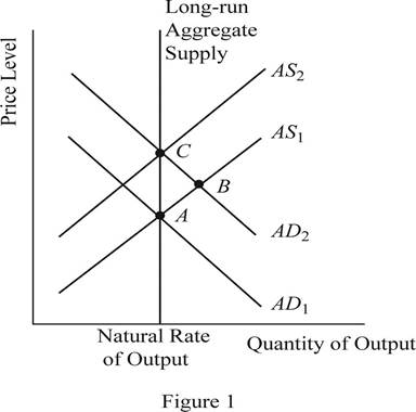
The equilibrium is a condition where the aggregate demand curve of the economy intersects with the aggregate supply curve of the economy. Then there will be an equilibrium point derived where the economy will be in its equilibrium without any excess demand or supply. The quantity on the X axis will represent the
Concept introduction:
Aggregate demand curve: It is the curve which shows the relationship between the price level in the economy and the quantity of real GDP demanded by the economic agents such as the households, firms as well as the government.
Equilibrium: The equilibrium in the economy is the point where the economy's aggregate demand curve and the aggregate supply curve intersects with each other. There will be no excess demand or
Subpart (b):
Long run equilibrium in AD-AS model.
Subpart (b):
Explanation of Solution
When the money supply of the economy increases with the intervention of the Central Bank of the economy, the money with the public will increase. When the money with the public increases, they will feel wealthier and as a result they will demand more consumer goods and services. As a result, the aggregate demand of the economy increases and it will shift the AD curve towards the right. This can be identified as the change to the equilibrium point B as shown in Figure 1. Thus, in short, the increase in the money supply leads to the increase in the output and price level of the economy.
Concept introduction:
Aggregate demand curve: It is the curve which shows the relationship between the price level in the economy and the quantity of real GDP demanded by the economic agents such as the households, firms as well as the government.
Aggregate supply curve: In the short run, it is a curve which shows the relationship between the price level in the economy and the supply in the economy by the firms. In the long run, it shows the relationship between the price level and the level of quantity supplied by the firms.
Equilibrium: The equilibrium in the economy is the point where the economy's aggregate demand curve and the aggregate supply curve intersects with each other. There will be no excess demand or excess supply in the economy at the equilibrium.
Subpart (c):
Long run equilibrium in AD-AS model.
Subpart (c):
Explanation of Solution
When the AD curve shifts towards the right and increases the output and the price level in the short run, over time, the nominal wages, prices as well as the perceptions and expectations of the economy would adjust to the new equilibrium level. As a result of this gradual adjustment, the cost of production will increase and the result will be a leftward shift in the aggregate supply curve of the economy. Then the economy will return to its natural level of output at a higher price level of the economy. This can be identified as the movement from point B to point C in the graph shown above.
Concept introduction:
Aggregate demand curve: It is the curve which shows the relationship between the price level in the economy and the quantity of real GDP demanded by the economic agents such as the households, firms as well as the government.
Aggregate supply curve: In the short run, it is a curve which shows the relationship between the price level in the economy and the supply in the economy by the firms. In the long run, it shows the relationship between the price level and the level of quantity supplied by the firms.
Equilibrium: The equilibrium in the economy is the point where the economy's aggregate demand curve and the aggregate supply curve intersects with each other. There will be no excess demand or excess supply in the economy at the equilibrium.
Subpart (d):
Long run equilibrium in AD-AS model.
Subpart (d):
Explanation of Solution
The sticky wages theory suggests that when there is inflation in the economy, the wage rate will adjust very slowly to the inflation. More or less the wage rates will be sticky and the main reason will be the long term contracts between the employer and the employees. Thus, in the short run equilibriums such as point A and point B, the wages of the economy would be more or less equal to each other. Whereas the point C represents the long run equilibrium and thus, the wages at the point C will be higher than that in point A and B.
Concept introduction:
Aggregate demand curve: It is the curve which shows the relationship between the price level in the economy and the quantity of real GDP demanded by the economic agents such as the households, firms as well as the government.
Aggregate supply curve: In the short run, it is a curve which shows the relationship between the price level in the economy and the supply in the economy by the firms. In the long run, it shows the relationship between the price level and the level of quantity supplied by the firms.
Equilibrium: The equilibrium in the economy is the point where the economy's aggregate demand curve and the aggregate supply curve intersects with each other. There will be no excess demand or excess supply in the economy at the equilibrium.
Subpart (e):
Long run equilibrium in AD-AS model.
Subpart (e):
Explanation of Solution
The sticky wages theory suggests that when there is inflation in the economy, the wage rate will adjust very slowly to the inflation. More or less, the wage rates will be sticky and the main reason will be the long term contracts between the employer and the employees. So, the nominal wages at equilibrium point A and B will be same. But the increase in the general price level in the economy would reduce the real wages of the workers because, the real wage is the nominal wage divided by the price level. When the denominator increases, it will reduce the value of the real wages in the economy.
Concept introduction:
Aggregate demand curve: It is the curve which shows the relationship between the price level in the economy and the quantity of real GDP demanded by the economic agents such as the households, firms as well as the government.
Aggregate supply curve: In the short run, it is a curve which shows the relationship between the price level in the economy and the supply in the economy by the firms. In the long run, it shows the relationship between the price level and the level of quantity supplied by the firms.
Equilibrium: The equilibrium in the economy is the point where the economy's aggregate demand curve and the aggregate supply curve intersects with each other. There will be no excess demand or excess supply in the economy at the equilibrium.
Sub part (f):
Long run equilibrium in AD-AS model.
Sub part (f):
Explanation of Solution
When the increase in the money supply happens in the economy, it will lead to the increase in the nominal wages as well as the price level in the economy in the long run. As a result of the increase in the nominal wage rate along with the price level in the economy, the real wage rate of the economy would remain unchanged. Thus, the neutrality of money applies in the long run equilibrium.
Concept introduction:
Aggregate demand curve: It is the curve which shows the relationship between the price level in the economy and the quantity of real GDP demanded by the economic agents such as the households, firms as well as the government.
Aggregate supply curve: In the short run, it is a curve which shows the relationship between the price level in the economy and the supply in the economy by the firms. In the long run, it shows the relationship between the price level and the level of quantity supplied by the firms.
Equilibrium: The equilibrium in the economy is the point where the economy's aggregate demand curve and the aggregate supply curve intersects with each other. There will be no excess demand or excess supply in the economy at the equilibrium.
Want to see more full solutions like this?
Chapter 33 Solutions
Principles of Economics

- How does the mining industry in canada contribute to the Canadian economy? Describe why your industry is so important to the Canadian economy What would happen if your industry disappeared, or suffered significant layoffs?arrow_forwardWhat is already being done to make mining in canada more sustainable? What efforts are being made in order to make mining more sustainable?arrow_forwardWhat are the environmental challenges the canadian mining industry face? Discuss current challenges that mining faces with regard to the environmentarrow_forward
- What sustainability efforts have been put forth in the mining industry in canada Are your industry’s resources renewable or non-renewable? How do you know? Describe your industry’s reclamation processarrow_forwardHow does oligopolies practice non-price competition in South Africa?arrow_forwardWhat are the advantages and disadvantages of oligopolies on the consumers, businesses and the economy as a whole?arrow_forward
- 1. After the reopening of borders with mainland China following the COVID-19 lockdown, residents living near the border now have the option to shop for food on either side. In Hong Kong, the cost of food is at its listed price, while across the border in mainland China, the price is only half that of Hong Kong's. A recent report indicates a decline in food sales in Hong Kong post-reopening. ** Diagrams need not be to scale; Focus on accurately representing the relevant concepts and relationships rather than the exact proportions. (a) Using a diagram, explain why Hong Kong's food sales might have dropped after the border reopening. Assume that consumers are indifferent between purchasing food in Hong Kong or mainland China, and therefore, their indifference curves have a slope of one like below. Additionally, consider that there are no transport costs and the daily food budget for consumers is identical whether they shop in Hong Kong or mainland China. I 3. 14 (b) In response to the…arrow_forward2. Health Food Company is a well-known global brand that specializes in healthy and organic food products. One of their main products is organic chicken, which they source from small farmers in the area. Health Food Company is the sole buyer of organic chicken in the market. (a) In the context of the organic chicken industry, what type of market structure is Health Food Company operating in? (b) Using a diagram, explain how the identified market structure affects the input pricing and output decisions of Health Food Company. Specifically, include the relevant curves and any key points such as the profit-maximizing price and quantity. () (c) How can encouraging small chicken farmers to form bargaining associations help improve their trade terms? Explain how this works by drawing on the graph in answer (b) to illustrate your answer.arrow_forward2. Suppose that a farmer has two ways to produce his crop. He can use a low-polluting technology with the marginal cost curve MCL or a high polluting technology with the marginal cost curve MCH. If the farmer uses the high-polluting technology, for each unit of quantity produced, one unit of pollution is also produced. Pollution causes pollution damages that are valued at $E per unit. The good produced can be sold in the market for $P per unit. P 1 MCH 0 Q₁ MCL Q2 E a. b. C. If there are no restrictions on the firm's choices, which technology will the farmer use and what quantity will he produce? Explain, referring to the area identified in the figure Given your response in part a, is it socially efficient for there to be no restriction on production? Explain, referring to the area identified in the figure If the government restricts production to Q1, what technology would the farmer choose? Would a socially efficient outcome be achieved? Explain, referring to the area identified in…arrow_forward
- I need help in seeing how these are the answers. If you could please write down your steps so I can see how it's done please.arrow_forwardSuppose that a random sample of 216 twenty-year-old men is selected from a population and that their heights and weights are recorded. A regression of weight on height yields Weight = (-107.3628) + 4.2552 x Height, R2 = 0.875, SER = 11.0160 (2.3220) (0.3348) where Weight is measured in pounds and Height is measured in inches. A man has a late growth spurt and grows 1.6200 inches over the course of a year. Construct a confidence interval of 90% for the person's weight gain. The 90% confidence interval for the person's weight gain is ( ☐ ☐) (in pounds). (Round your responses to two decimal places.)arrow_forwardSuppose that (Y, X) satisfy the assumptions specified here. A random sample of n = 498 is drawn and yields Ŷ= 6.47 + 5.66X, R2 = 0.83, SER = 5.3 (3.7) (3.4) Where the numbers in parentheses are the standard errors of the estimated coefficients B₁ = 6.47 and B₁ = 5.66 respectively. Suppose you wanted to test that B₁ is zero at the 5% level. That is, Ho: B₁ = 0 vs. H₁: B₁ #0 Report the t-statistic and p-value for this test. Definition The t-statistic is (Round your response to two decimal places) ☑ The Least Squares Assumptions Y=Bo+B₁X+u, i = 1,..., n, where 1. The error term u; has conditional mean zero given X;: E (u;|X;) = 0; 2. (Y;, X¡), i = 1,..., n, are independent and identically distributed (i.i.d.) draws from i their joint distribution; and 3. Large outliers are unlikely: X; and Y, have nonzero finite fourth moments.arrow_forward
 Essentials of Economics (MindTap Course List)EconomicsISBN:9781337091992Author:N. Gregory MankiwPublisher:Cengage Learning
 Principles of Economics (MindTap Course List)EconomicsISBN:9781305585126Author:N. Gregory MankiwPublisher:Cengage Learning
 Principles of Macroeconomics (MindTap Course List)EconomicsISBN:9781285165912Author:N. Gregory MankiwPublisher:Cengage Learning
 Brief Principles of Macroeconomics (MindTap Cours...EconomicsISBN:9781337091985Author:N. Gregory MankiwPublisher:Cengage Learning
 Principles of Economics, 7th Edition (MindTap Cou...EconomicsISBN:9781285165875Author:N. Gregory MankiwPublisher:Cengage Learning
 Principles of Macroeconomics (MindTap Course List)EconomicsISBN:9781305971509Author:N. Gregory MankiwPublisher:Cengage Learning