Concept explainers
Video Games and Grade-Point Average Professor Grant Alexander wanted to find a linear model that relates the number of hours a student plays video games each week. , to the cumulative grade-point average. , of the student. He obtained a random sample of 10 full-time students at his college and asked each student to disclose the number of hours spent playing video games and the student’s cumulative grade-point average.
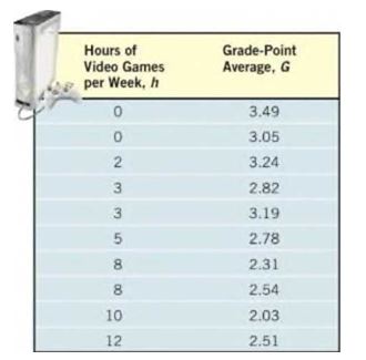
(a) Explain why the number of hours spent playing video games is the independent variable and cumulative grade-point average is the dependent variable.
(b) Use a graphing utility to draw a
(c) Use a graphing utility to find the line of best fit that models the relation between number of hours of video game playing each week and grade-point average. Express the model using function notation.
(d) Interpret the slope.
(e) Predict the grade-point average of a student who plays video games for 8 hours each week.
(f) How many hours of video game playing do you think a student plays whose grade-point average is ?
Want to see the full answer?
Check out a sample textbook solutionChapter 3 Solutions
Precalculus
Additional Math Textbook Solutions
University Calculus: Early Transcendentals (4th Edition)
Thomas' Calculus: Early Transcendentals (14th Edition)
Calculus and Its Applications (11th Edition)
Calculus, Single Variable: Early Transcendentals (3rd Edition)
Calculus: Early Transcendentals (3rd Edition)
- Does Table 1 represent a linear function? If so, finda linear equation that models the data.arrow_forwardIf you travel 100 miles in two hours, then your average speed for the trip is Average speed=_________=________arrow_forwardIn a certain country, total alcoholic beverage sales are reported throughout the year. Sales were reported as $118.5 billion at the beginning of 2004 and $136.2 billion at the beginning of 2006. (a) Let the x-axis denote time and the y-axis denote the amount of alcohol sales (in billions), Let x = 0 correspond to 2004. Fill in the blanks: The given data is represented by the points ( 118.5) and (2, ). (b) Find the linear equation determined by the two points in part (a). (c) Use the equation in part (b) to estimate the alcohol sales produced in 2005. (d) If the model remains accurate, in what year will reported alcohol sales reach $150 billion? (a) The given data is represented by the points (,118.5) and (2,). (Type integers decimals rounded to one decimal place.) (b) The linear equation determined by the two points in part (a) is y =x+. (Type integers or decimals rounded to one decimal place.) (c) The alcohol sales produced in 2005 are approximately $ billion. (Type an integer or…arrow_forward
- To investigate the relationship between yield of soybeans and the amount of fertilizer used, a researcher divides a field into eight plots of equal size and applies a different amount of fertilizer to each plot. The table shows the yield of soybeans and the amount of fertilizer used for each plot. A scatterplot of the data confirms that there is a linear association. Predict the yield of soybeans for 2.75 pounds of fertilizer. Round answer to the nearest whole number. Do not include the label in your answer. Amount of Fertilizer (in pounds) Yield of soybeans (in pounds) 1 25 1.5 21 2 27 2.5 28 3 36 3.5 35 4 32 4.5 34 im not sure how to start with thisarrow_forwardDo heavier cars use more gasoline? To answer this question, a researcher randomly selected 15 cars. He collected their weight (in hundreds of pounds) and the mileage (MPG) for each car. From a scatterplot made with the data, a linear model seemed appropriate which is included as a photo. What proportion of the variation in mileage is accounted for by the linear relationship with the wight of the car? And if we wanted to test if there is a significant straight-line relationship between the weight and the mileage of a car, we can perform a T test. Give the value of the t statistic for this test.arrow_forwardA magazine publishes restaurant ratings for various locations around the world. The magazine rates the restaurants for food, decor, service, and the cost per person. Develop a regression model to predict the cost per person, based on a variable that represents the sum of the three ratings. The magazine has compiled the accompanying table of this summated ratings variable and the cost per person for 25 restaurants in a major city. Complete parts (a) through (e) below. Click the icon to view the table of summated ratings and cost per person. ..... a. Construct a scatter plot. Choose the correct graph below. A. Ов. С. D. ACost ($) 90- ACost ($) 90- ACost ($) 90- ACost ($) 90- 0- 0- 90 90 90 90 Rating Rating Rating Rating b. Assuming a linear relationship, use the least-squares method to compute the regression coefficients b, and b,. bo = and b, (Round to two decimal places as needed.) c. Interpret the meaning of the Y-intercept, bo, and the slope, b,. Choose the correct answer below. O A.…arrow_forward
- A magazine publishes restaurant ratings for various locations around the world. The magazine rates the restaurants for food, decor, service, and the cost per person. Develop a regression model to predict the cost per person, based on a variable that represents the sum of the three ratings. The magazine has compiled the accompanying table of this summated ratings variable and the cost per person for 25 restaurants in a major city. Complete parts (a) through (e) below. Click the icon to view the table of summated ratings and cost per person. a. Construct a scatter plot. Choose the correct graph below. O A. 90+ 0 0 Cost ($) The M Rating 90 Q O B. A Cost (5) 90+ 0 H +4 Alpe Rating 90 Q b. Assuming a linear relationship, use the least-squares method to compute the regression coefficients bo and b₁. bo= and b₁ = (Round to two decimal places as needed.) C O C. 90+ 0- Cost (S) HA Rating 90 Q Summated Ratings and Cost Per Person Summated Rating Cost ($ per person) 40 48 60 61 42 40 43 55 67 69…arrow_forwardA magazine publishes restaurant ratings for various locations around the world. The magazine rates the restaurants for food, decor, service, and the cost per person. Develop a regression model to predict the cost per person, based on a variable that represents the sum of the three ratings. The magazine has compiled the accompanying table of this summated ratings variable and the cost per person for 25 restaurants in a major city. Complete parts (a) through (e) below. Click the icon to view the table of summated ratings and cost per person. a. Construct a scatter plot. Choose the correct graph below. O A. Ов. OC. OD. ACost ($) 90- Q A Cost ($) 904 A Cost ($) 90- ACost ($) 90- 0- 0- 0- 0- 90 Rating 90 Rating 90 90 Rating Rating Summated ratings and cost per person b. Assuming a linear relationship, use the least-squares method to compute the regression coefficients bo and b,. bo =D and b, =O (Round to two decimal places as needed.) Summated Rating Cost ($ per person)|9 c. Interpret the…arrow_forwardHow wide is the chasm between what men and women earn in the workplace? According to a 2015 analysis from a national women's group, women lose $435,049 over the course of a career because of the pay gap. The bar graph to the right shows the average earnings in the United States for men and women at ages 22 and 55. This exercise involves the graphs of models for the data shown in the rectangular coordinate system to the right. Complete parts (a) through (c) below. BEEB Average Yearly Earnings in the U.S., by Gender and Age M(age=33)=$thousand (Type an integer or decimal rounded to one decimal place as needed.) Average Yearly Earnings ($1000s) 70- 60- Men 50-Women- 40- 30- 20- 10- 0- 22 Age 55 Average Yearly Earnings ($1000s) A $70 (3087) $60- $30 $20- $10- $0 } e $50 (0.23) $40 BN 9 ST (Use integers or decimals for any numbers in the expression. Round to two decimal places as needed.) b. Use the two points for women shown on the graph to find a function in the form W(x) = mx + b that…arrow_forward
- How wide is the chasm between what men and women earn in the workplace? According to a 2015 analysis from a national women's group, women lose $435,049 over the course of a career because of the pay gap. The bar graph to the right shows the average earnings in the United States for men and women at ages 22 and 60. This exercise involves the graphs of models for the data shown in the rectangular coordinate system to the right. Complete parts (a) through (c) below. Average Yearly Earnings ($1000s) Average Yearly Earnings in the U.S., by Gender and Age 70- 60- ■Men 50 Women 40- 30- 20- 10- 0- 22 Age 60 Average Yearly Earnings ($1000s) $70- $60- (30,67).. $50 (0,24) $40+ $30+ $20- $10- $0+ 0 M(age=38) = $ thousand (Type an integer or decimal rounded to one decimal place as needed.) ♦ (0,21) Men *(30,40) Women 10 20 30 40 50 Years after Age 22 --X7 (Use integers or decimals for any numbers in the expression. Round to two decimal places as needed.) b. Use the two points for women shown on…arrow_forwardA random sample of 136 adults were asked to report the number of hours per week the spent on a computer and their number of years of education. The linear model equation below describes the relationship between the mean computers hours and years of education. computers == 9.12 ++ 0.8 ×× education Based on this linear model, which of the following statements is correct? a) An adult who has no years of education is expected to spend 9.12 hours per week on a computer. b) An adult who has 1 more year of education than another is expected to spend 9.12 more hours per week on a computer. c) An adult who spends 1 more hour per week on a computer than another is expected to have had 9.12 more years of education. d) An adult who spend zero hours per week on a computer is expected to have 9.12 years of education.arrow_forwardOne of the biggest changes in higher education in recent years has been the growth of online universities. The Online Education Database is an independent organization whose mission is to build a comprehensive list of the top accredited online colleges. The following table shows the retention rate (%) and the graduation rate (%) for 29 online colleges.a). Use Excel Data Analysis Tool – Regression to get the relationship between the two variables;b). Create a scatter diagram for the two variables and display regression equation and R square on chart, then explain the relationship between the variables;c). Did the estimated regression equation provide a good fit?d). Suppose you were the president of South University. After reviewing the results, would you be able to use the regression result for forecasting. College RR(%) GR(%) Western International University 7 25 South University 51 25 University of Phoenix 4 28 American InterContinental University 29 32 Franklin…arrow_forward
- Glencoe Algebra 1, Student Edition, 9780079039897...AlgebraISBN:9780079039897Author:CarterPublisher:McGraw HillHolt Mcdougal Larson Pre-algebra: Student Edition...AlgebraISBN:9780547587776Author:HOLT MCDOUGALPublisher:HOLT MCDOUGAL
- Big Ideas Math A Bridge To Success Algebra 1: Stu...AlgebraISBN:9781680331141Author:HOUGHTON MIFFLIN HARCOURTPublisher:Houghton Mifflin HarcourtCollege AlgebraAlgebraISBN:9781305115545Author:James Stewart, Lothar Redlin, Saleem WatsonPublisher:Cengage Learning