
Sub part (a):
Consumption schedule and marginal propensity to consume.
Sub part (a):
Explanation of Solution
Table -1 shows the consumption schedule:
Table -1
| Consumption | |
| 100 | 120 |
| 200 | 200 |
| 300 | 280 |
| 400 | 360 |
| 500 | 440 |
| 600 | 520 |
| 700 | 600 |
Figure 1 illustrates the level of consumption at different level of gross domestic product (GDP).
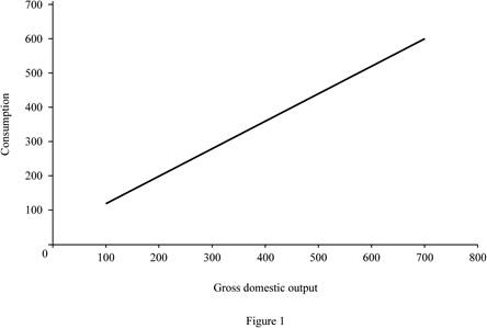
In Figure 1, the horizontal axis measures the gross domestic output and the vertical axis measures the consumption level.
Size of marginal propensity to consume (MPC) can be calculated as follows.
The size of marginal propensity to consume is 0.8.
Concept introduction:
Consumption schedule: Consumption schedule refers to the quantity of consumption at different levels of income.
Marginal propensity to consume (MPS): Marginal propensity to consume refers to the sensitivity of change in the consumption level due to the changes occurred in the income level.
Sub part (b):
Disposable income, tax rate, consumption schedule, marginal propensity to consume and multiplier.
Sub part (b):
Explanation of Solution
Disposable income (DI) can be calculated by using the following formula.
Substitute the respective values in Equation (1) to calculate the disposable income at the level of GDP $100.
Disposable income at the level of GDP $100 is $90.
Tax rate can be calculated by using the following formula.
Substitute the respective values in Equation (2) to calculate the tax rate at the level of GDP $100.
Tax rate at the level of GDP is 10%.
New consumption level can be calculated by using the following formula.
Substitute the respective values in Equation (3) to calculate the disposable income at the level of GDP $100. Since, the tax payment is equal amount of decrease in consumption for all the levels of GDP. The decreasing consumption for increasing $10 is assumed to be $8.
New consumption is $112.
Table -2 shows the values of disposable income, new consumption level after tax and the tax rate that are obtained by using Equations (1), (2) and (3).
Table -2
| Gross domestic product | Tax | DI | New consumption | Tax rate |
| 100 | 10 | 90 | 112 | 10% |
| 200 | 10 | 190 | 192 | 5% |
| 300 | 10 | 290 | 272 | 3.33% |
| 400 | 10 | 390 | 352 | 2.5% |
| 500 | 10 | 490 | 432 | 2% |
| 600 | 10 | 590 | 512 | 1.67% |
| 700 | 10 | 690 | 592 | 1.43% |
Size of marginal propensity to consume (MPC) can be calculated as follows.
The size of marginal propensity to consume is 0.8.
Multiplier: Multiplier refers to the ratio of change in the real GDP to the change in initial consumption, at a constant price rate. Multiplier is positively related to the marginal propensity to consumer and negatively related with the marginal propensity to save. Multiplier can be evaluated using the following formula:
Since the value of MPC remains the same for part (a) and part (b), there is no change in the value of multiplier. The value of multiplier is 5
Figure -2 illustrates the level of consumption at different level of gross domestic product (GDP) for lump sum tax (Regressive tax).
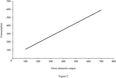
In Figure -2, the horizontal axis measures the gross domestic output and the vertical axis measures the consumption level.
Concept introduction:
Consumption schedule: Consumption schedule refers to the quantity of consumption at different levels of income.
Marginal propensity to consume (MPS): Marginal propensity to consume refers to the sensitivity of change in the consumption level due to the changes occurred in the income level.
Multiplier: Multiplier refers to the ratio of change in the real GDP to the change in initial consumption at constant price rate. Multiplier is positively related to the marginal propensity to consumer and negatively related with the marginal propensity to save.
Sub part (c):
Tax amount, consumption schedule, marginal propensity to consume and multiplier.
Sub part (c):
Explanation of Solution
Tax amount can be calculated by using the following formula.
Substitute the respective values in Equation (4) to calculate the tax amount at $100 GDP.
Tax amount is $10.
Table -3 shows the values of disposable income, new consumption level after tax and the tax rate that are obtained by using Equations (1), (2), (3) and (4). The change in tax amount is differing for different levels of GDP. The decreasing consumption for increasing each $10 is assumed to be $8 (Thus, if the tax payment is $30, then the consumption decreases by $24
Table -3
| Gross domestic product | Tax | DI | New consumption | Tax rate |
| 100 | 10 | 90 | 112 | 10% |
| 200 | 20 | 180 | 184 | 10% |
| 300 | 30 | 270 | 256 | 10% |
| 400 | 40 | 360 | 328 | 10% |
| 500 | 50 | 450 | 400 | 10% |
| 600 | 60 | 540 | 472 | 10% |
| 700 | 70 | 630 | 544 | 10% |
Multiplier: Multiplier refers to the ratio of change in the real GDP to the change in initial consumption, at a constant price rate. Multiplier is positively related to the marginal propensity to consumer and negatively related with the marginal propensity to save. Multiplier can be evaluated using the following formula:
Since the value of MPC different for part (a) and part (c), the value of multiplier for both the part is different. The value of multiplier is 3.57
Figure -3 illustrates the level of consumption at different level of gross domestic product (GDP) for proportional tax.
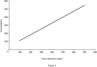
In Figure -3, the horizontal axis measures the gross domestic output and the vertical axis measures the consumption level.
Concept introduction:
Consumption schedule: Consumption schedule refers to the quantity of consumption at different levels of income.
Marginal propensity to consume (MPS): Marginal propensity to consume refers to the sensitivity of change in the consumption level due to the changes occurred in the income level.
Multiplier: Multiplier refers to the ratio of change in the real GDP to the change in initial consumption at constant price rate. Multiplier is positively related to the marginal propensity to consumer and negatively related with the marginal propensity to save.
Sub part (d):
consumption schedule, marginal propensity to consume and multiplier.
Sub part (d):
Explanation of Solution
Marginal propensity to consume can be calculated by using the following formula.
Substitute the respective values in Equation (5) to calculate the MPC at $100 GDP.
The value of MPC is 0.72.
Table -4 shows the values of disposable income, new consumption level after tax and the tax rate that are obtained by using Equations (1), (2), (3), (4) and (5). The change in tax amount is differing for different levels of GDP. The decreasing consumption for increasing each $10 is assumed to be $8 (Thus, if the tax payment is $20, then the consumption decreases by $16
Table -3
| Gross domestic product | Tax | DI | New consumption | Tax rate | MPC |
| 100 | 0 | 100 | 120 | 0% | |
| 200 | 10 | 190 | 192 | 5% | 0.8 |
| 300 | 30 | 270 | 256 | 10% | 0.64 |
| 400 | 60 | 340 | 312 | 15% | 0.56 |
| 500 | 100 | 400 | 360 | 20% | 0.48 |
| 600 | 150 | 450 | 400 | 25% | 0.4 |
| 700 | 210 | 490 | 432 | 30% | 0.32 |
Multiplier: Multiplier refers to the ratio of change in the real GDP to the change in initial consumption, at a constant price rate. Multiplier is positively related to the marginal propensity to consumer and negatively related with the marginal propensity to save.
Multiplier value is differing for each level of GDP. When the tax rate increases, it reduces the value of MPC. Since the value of MPC decreases, the value of multiplier will also decrease.
Figure 4 illustrates the level of consumption at different level of gross domestic product (GDP) for progressive tax.
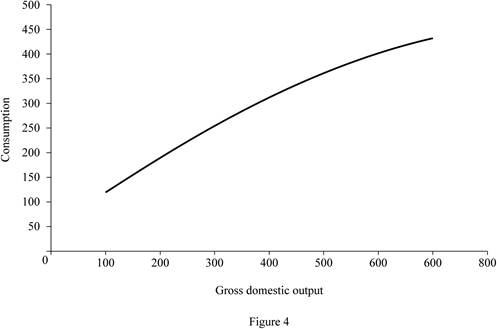
In Figure 4, the horizontal axis measures the gross domestic output and the vertical axis measures the consumption level.
Concept introduction:
Consumption schedule: Consumption schedule refers to the quantity of consumption at different levels of income.
Marginal propensity to consume (MPS): Marginal propensity to consume refers to the sensitivity of change in the consumption level due to the changes occurred in the income level.
Multiplier: Multiplier refers to the ratio of change in the real GDP to the change in initial consumption at constant price rate. Multiplier is positively related to the marginal propensity to consumer and negatively related with the marginal propensity to save.
Sup part (e):
Marginal propensity to consume and multiplier.
Sup part (e):
Explanation of Solution
Figure 1, Figure 2, Figure 3 and Figure 4 reveals that the proportional and progressive tax system reduces the value of MPC, so that the value of multiplier also decreases. The regressive tax system (Lump sum tax) does not alter the MPC. Since there is no change in the MPC, the multiplier remains the same.
Concept introduction:
Marginal propensity to consume (MPS): Marginal propensity to consume refers to the sensitivity of change in the consumption level due to the changes occurred in the income level.
Progressive tax: Progressive tax refers to the higher income people paying higher tax amount than the lower income people.
Proportional tax: Proportional tax rate refers to the fixed tax rate regardless of income and the tax rate and is the same for all levels of income.
Regressive tax: Regressive tax refers to the higher income people paying lower percentage of tax amount and lower income people paying higher percentage of tax amount.
Multiplier: Multiplier refers to the ratio of change in the real GDP to the change in initial consumption at constant price rate. Multiplier is positively related to the marginal propensity to consumer and negatively related with the marginal propensity to save.
Want to see more full solutions like this?

- Please help me with this Accounting questionarrow_forwardTitle: Does the educational performance depend on its literacy rate and government spending over the last 10 years? In the introduction, there are four things to include:a) Clearly state your research topic follows by country’s background in terms of (population density; male/female ratio; and identify the problem leading up to the study of it, such as government spending and adult literacy rate. How does the US perform compared to other countries.b) State the research question that you wish to resolve: Does the US economic performance depend on its government spending on education and the literacy rate over the last 10 years. Define performance (Y) as the average income per capita, an indicator of the country’s economy growing over time. For example, an increase in government spending leads to higher literacy rates and subsequently higher productivity in the economy. Also, mention that you will use a sample size of 10 years of secondary data from the existing literature,…arrow_forwardTitle: Does the educational performance depend on its literacy rate and government spending over the last 10 years? In the introduction, there are four things to include:a) Clearly state your research topic follows by country’s background in terms of (population density; male/female ratio; and identify the problem leading up to the study of it, such as government spending and adult literacy rate. How does the US perform compared to other countries.b) State the research question that you wish to resolve: Does the US economic performance depend on its government spending on education and the literacy rate over the last 10 years. Define performance (Y) as the average income per capita, an indicator of the country’s economy growing over time. For example, an increase in government spending leads to higher literacy rates and subsequently higher productivity in the economy. Also, mention that you will use a sample size of 10 years of secondary data from the existing literature,…arrow_forward
- Explain how the introduction of egg replacers and plant-based egg products will impact the bakery industry. Provide a graphical representation.arrow_forwardExplain Professor Frederick's "cognitive reflection" test.arrow_forward11:44 Fri Apr 4 Would+You+Take+the+Bird+in+the+Hand Would You Take the Bird in the Hand, or a 75% Chance at the Two in the Bush? BY VIRGINIA POSTREL WOULD you rather have $1,000 for sure or a 90 percent chance of $5,000? A guaranteed $1,000 or a 75 percent chance of $4,000? In economic theory, questions like these have no right or wrong answers. Even if a gamble is mathematically more valuable a 75 percent chance of $4,000 has an expected value of $3,000, for instance someone may still prefer a sure thing. People have different tastes for risk, just as they have different tastes for ice cream or paint colors. The same is true for waiting: Would you rather have $400 now or $100 every year for 10 years? How about $3,400 this month or $3,800 next month? Different people will answer differently. Economists generally accept those differences without further explanation, while decision researchers tend to focus on average behavior. In decision research, individual differences "are regarded…arrow_forward
- Describe the various measures used to assess poverty and economic inequality. Analyze the causes and consequences of poverty and inequality, and discuss potential policies and programs aimed at reducing them, assess the adequacy of current environmental regulations in addressing negative externalities. analyze the role of labor unions in labor markets. What is one benefit, and one challenge associated with labor unions.arrow_forwardEvaluate the effectiveness of supply and demand models in predicting labor market outcomes. Justify your assessment with specific examples from real-world labor markets.arrow_forwardExplain the difference between Microeconomics and Macroeconomics? 2.) Explain what fiscal policy is and then explain what Monetary Policy is? 3.) Why is opportunity cost and give one example from your own of opportunity cost. 4.) What are models and what model did we already discuss in class? 5.) What is meant by scarcity of resources?arrow_forward
- 2. What is the payoff from a long futures position where you are obligated to buy at the contract price? What is the payoff from a short futures position where you are obligated to sell at the contract price?? Draw the payoff diagram for each position. Payoff from Futures Contract F=$50.85 S1 Long $100 $95 $90 $85 $80 $75 $70 $65 $60 $55 $50.85 $50 $45 $40 $35 $30 $25 Shortarrow_forward3. Consider a call on the same underlier (Cisco). The strike is $50.85, which is the forward price. The owner of the call has the choice or option to buy at the strike. They get to see the market price S1 before they decide. We assume they are rational. What is the payoff from owning (also known as being long) the call? What is the payoff from selling (also known as being short) the call? Payoff from Call with Strike of k=$50.85 S1 Long $100 $95 $90 $85 $80 $75 $70 $65 $60 $55 $50.85 $50 $45 $40 $35 $30 $25 Shortarrow_forward4. Consider a put on the same underlier (Cisco). The strike is $50.85, which is the forward price. The owner of the call has the choice or option to buy at the strike. They get to see the market price S1 before they decide. We assume they are rational. What is the payoff from owning (also known as being long) the put? What is the payoff from selling (also known as being short) the put? Payoff from Put with Strike of k=$50.85 S1 Long $100 $95 $90 $85 $80 $75 $70 $65 $60 $55 $50.85 $50 $45 $40 $35 $30 $25 Shortarrow_forward
 Principles of Economics 2eEconomicsISBN:9781947172364Author:Steven A. Greenlaw; David ShapiroPublisher:OpenStax
 Principles of Economics (MindTap Course List)EconomicsISBN:9781305585126Author:N. Gregory MankiwPublisher:Cengage Learning
 Principles of Macroeconomics (MindTap Course List)EconomicsISBN:9781285165912Author:N. Gregory MankiwPublisher:Cengage Learning
 Brief Principles of Macroeconomics (MindTap Cours...EconomicsISBN:9781337091985Author:N. Gregory MankiwPublisher:Cengage Learning
 Principles of Economics, 7th Edition (MindTap Cou...EconomicsISBN:9781285165875Author:N. Gregory MankiwPublisher:Cengage Learning