
Essential Statistics
2nd Edition
ISBN: 9781259570643
Author: Navidi
Publisher: MCG
expand_more
expand_more
format_list_bulleted
Concept explainers
Videos
Textbook Question
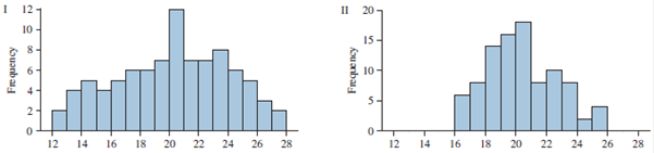
Chapter 3, Problem 7CQ
Each of the following histograms represents a data set with
Expert Solution & Answer
Want to see the full answer?
Check out a sample textbook solution
Students have asked these similar questions
please find the answers for the yellows boxes using the information and the picture below
A marketing agency wants to determine whether different advertising platforms generate significantly different levels of customer engagement. The agency measures the average number of daily clicks on ads for three platforms: Social Media, Search Engines, and Email Campaigns. The agency collects data on daily clicks for each platform over a 10-day period and wants to test whether there is a statistically significant difference in the mean number of daily clicks among these platforms. Conduct ANOVA test.
You can provide your answer by inserting a text box and the answer must include: also please provide a step by on getting the answers in excel
Null hypothesis,
Alternative hypothesis,
Show answer (output table/summary table), and
Conclusion based on the P value.
A company found that the daily sales revenue of its flagship product follows a normal distribution with a mean of $4500 and a standard deviation of $450. The company defines a "high-sales day" that is, any day with sales exceeding $4800. please provide a step by step on how to get the answers
Q: What percentage of days can the company expect to have "high-sales days" or sales greater than $4800?
Q: What is the sales revenue threshold for the bottom 10% of days? (please note that 10% refers to the probability/area under bell curve towards the lower tail of bell curve)
Provide answers in the yellow cells
Chapter 3 Solutions
Essential Statistics
Ch. 3.1 - 1. Compute the mean and median of the following...Ch. 3.1 - 2. Compute the mean and median of the following...Ch. 3.1 - Prob. 3CYUCh. 3.1 - Prob. 4CYUCh. 3.1 - 5. A data set has a mean of 5 and a median of 7....Ch. 3.1 - Prob. 6CYUCh. 3.1 - In Exercises 7–10, fill in each blank with the...Ch. 3.1 - In Exercises 7–10, fill in each blank with the...Ch. 3.1 - In Exercises 7–10, fill in each blank with the...Ch. 3.1 - In Exercises 7–10, fill in each blank with the...
Ch. 3.1 - Prob. 11ECh. 3.1 - Prob. 12ECh. 3.1 - Prob. 13ECh. 3.1 - Prob. 14ECh. 3.1 - Prob. 15ECh. 3.1 - Prob. 16ECh. 3.1 - Prob. 17ECh. 3.1 - 18. Find the mean, median, and mode for the...Ch. 3.1 - Prob. 19ECh. 3.1 - In Exercises 19–22, use the given frequency...Ch. 3.1 - Prob. 21ECh. 3.1 - In Exercises 19–22, use the given frequency...Ch. 3.1 - Prob. 23ECh. 3.1 - Prob. 24ECh. 3.1 - Prob. 25ECh. 3.1 - Prob. 26ECh. 3.1 - Prob. 27ECh. 3.1 - Prob. 28ECh. 3.1 - Prob. 29ECh. 3.1 - 30. Mean and median height: The National Center...Ch. 3.1 - 31. Hamburgers: An ABC News story reported the...Ch. 3.1 - Prob. 32ECh. 3.1 - Prob. 33ECh. 3.1 - Prob. 34ECh. 3.1 - Prob. 35ECh. 3.1 - 36. Beer: The following table presents the number...Ch. 3.1 - Prob. 37ECh. 3.1 - Prob. 38ECh. 3.1 - 39. Heavy football players: Following are the...Ch. 3.1 - Prob. 40ECh. 3.1 - Prob. 41ECh. 3.1 - 42. News flash: The following table presents the...Ch. 3.1 - Prob. 43ECh. 3.1 - Prob. 44ECh. 3.1 - Prob. 45ECh. 3.1 - Prob. 46ECh. 3.1 - Prob. 47ECh. 3.1 - Prob. 48ECh. 3.1 - Prob. 49ECh. 3.1 - Prob. 50ECh. 3.1 - Prob. 51ECh. 3.1 - 52. Sources of news: A sample of 32 U.S. adults...Ch. 3.1 - Prob. 53ECh. 3.1 - Prob. 54ECh. 3.1 - Prob. 55ECh. 3.1 - Prob. 56ECh. 3.1 - Prob. 57ECh. 3.1 - Prob. 58ECh. 3.1 - Prob. 59ECh. 3.1 - Prob. 60ECh. 3.1 - Prob. 61ECh. 3.1 - Prob. 62ECh. 3.1 - Prob. 63ECh. 3.1 - Prob. 64ECh. 3.1 - Prob. 65ECh. 3.1 - Prob. 66ECh. 3.1 - Prob. 67ECh. 3.1 - Prob. 68ECh. 3.1 - Prob. 69ECh. 3.1 - Prob. 70ECh. 3.1 - Prob. 71ECh. 3.1 - Prob. 72ECh. 3.1 - Prob. 73ECh. 3.1 - Prob. 74ECh. 3.2 - 1. Compute the population variance for the St....Ch. 3.2 - Prob. 2CYUCh. 3.2 - Prob. 3CYUCh. 3.2 - Prob. 4CYUCh. 3.2 - Prob. 5CYUCh. 3.2 - Prob. 6CYUCh. 3.2 - Prob. 7CYUCh. 3.2 - Prob. 8CYUCh. 3.2 - Prob. 9ECh. 3.2 - In Exercises 9–12, fill in each blank with the...Ch. 3.2 - Prob. 11ECh. 3.2 - In Exercises 9–12, fill in each blank with the...Ch. 3.2 - Prob. 13ECh. 3.2 - In Exercises 13–16, determine whether the...Ch. 3.2 - Prob. 15ECh. 3.2 - Prob. 16ECh. 3.2 - Prob. 17ECh. 3.2 - 18. Find the sample variance and standard...Ch. 3.2 - Prob. 19ECh. 3.2 - Prob. 20ECh. 3.2 - Prob. 21ECh. 3.2 - Prob. 22ECh. 3.2 - 23. Approximate the sample variance and standard...Ch. 3.2 - 24. Approximate the sample variance and standard...Ch. 3.2 - Prob. 25ECh. 3.2 - Prob. 26ECh. 3.2 - Prob. 27ECh. 3.2 - Prob. 28ECh. 3.2 - Prob. 29ECh. 3.2 - Prob. 30ECh. 3.2 - Prob. 31ECh. 3.2 - Prob. 32ECh. 3.2 - 33. Heavy football players: Following are the...Ch. 3.2 - 34. Beer: The following table presents the number...Ch. 3.2 - Prob. 35ECh. 3.2 - Prob. 36ECh. 3.2 - Prob. 37ECh. 3.2 - Prob. 38ECh. 3.2 - Prob. 39ECh. 3.2 - Prob. 40ECh. 3.2 - Prob. 41ECh. 3.2 - 42. Pay your bills: In a large sample of customer...Ch. 3.2 - Prob. 43ECh. 3.2 - Prob. 44ECh. 3.2 - Prob. 45ECh. 3.2 - 46. Pay your bills: For the data in Exercise 42,...Ch. 3.2 - Prob. 47ECh. 3.2 - 48. Internet providers: For the data in Exercise...Ch. 3.2 - Prob. 49ECh. 3.2 - Prob. 50ECh. 3.2 - Prob. 51ECh. 3.2 - Prob. 52ECh. 3.2 - Prob. 53ECh. 3.2 - Prob. 54ECh. 3.2 - Prob. 55ECh. 3.2 - Prob. 56ECh. 3.2 - Prob. 57ECh. 3.2 - Prob. 58ECh. 3.2 - Prob. 59ECh. 3.2 - Prob. 60ECh. 3.2 - Prob. 61ECh. 3.2 - Prob. 62ECh. 3.2 - Prob. 63ECh. 3.3 - Following are final exam scores, arranged in...Ch. 3.3 - Prob. 2CYUCh. 3.3 - Prob. 3CYUCh. 3.3 - Prob. 4CYUCh. 3.3 - Prob. 5ECh. 3.3 - In Exercises 5–8, fill in each blank with the...Ch. 3.3 - Prob. 7ECh. 3.3 - In Exercises 5–8, fill in each blank with the...Ch. 3.3 - Prob. 9ECh. 3.3 - In Exercises 9–12, determine whether the statement...Ch. 3.3 - Prob. 11ECh. 3.3 - Prob. 12ECh. 3.3 - A population has mean μ = 7 and standard deviation...Ch. 3.3 - Prob. 14ECh. 3.3 - Prob. 15ECh. 3.3 - Prob. 16ECh. 3.3 - Prob. 17ECh. 3.3 - Prob. 18ECh. 3.3 - Prob. 19ECh. 3.3 - For the data set a. Find the 80th percentile. b....Ch. 3.3 - Standardized tests: In a recent year, the mean...Ch. 3.3 - A fish story: The mean length of one-year-old...Ch. 3.3 - Prob. 23ECh. 3.3 - Blood pressure in women: The article referred to...Ch. 3.3 - Hazardous waste: Following is a list of the number...Ch. 3.3 - Cholesterol levels: The National Health and...Ch. 3.3 - Commuting to work: Jamie drives to work every...Ch. 3.3 - Windy city by the bay: Following are wind speeds...Ch. 3.3 - Caffeine: Following are the number of grams of...Ch. 3.3 - Nuclear power: The following table presents the...Ch. 3.3 - Place your bets: Recently, 28 states in the U.S....Ch. 3.3 - Hail to the chief: There have been 57 presidential...Ch. 3.3 - Prob. 33ECh. 3.3 - Prob. 34ECh. 3.3 - Prob. 35ECh. 3.3 - Automotive emissions: Following are levels of...Ch. 3.3 - Prob. 37ECh. 3.3 - Prob. 38ECh. 3.3 - Prob. 39ECh. 3.3 - Boxplot possible? Following is the five-number...Ch. 3.3 - Unusual boxplot: Ten residents of a town were...Ch. 3.3 - Prob. 42ECh. 3.3 - The vanishing outlier: Seven families live on a...Ch. 3.3 - Prob. 44ECh. 3.3 - Prob. 45ECh. 3 - Of the mean, median, and mode, which must be a...Ch. 3 - Prob. 2CQCh. 3 - Prob. 3CQCh. 3 - Prob. 4CQCh. 3 - Prob. 5CQCh. 3 - Prob. 6CQCh. 3 - Each of the following histograms represents a data...Ch. 3 - Prob. 8CQCh. 3 - Prob. 9CQCh. 3 - Prob. 10CQCh. 3 - Prob. 11CQCh. 3 - Prob. 12CQCh. 3 - Prob. 13CQCh. 3 - Prob. 14CQCh. 3 - Prob. 15CQCh. 3 - Prob. 1RECh. 3 - Prob. 2RECh. 3 - Prob. 3RECh. 3 - Prob. 4RECh. 3 - Prob. 5RECh. 3 - Prob. 6RECh. 3 - Measure that ball: Each of 16 students measured...Ch. 3 - Prob. 8RECh. 3 - Prob. 9RECh. 3 - How long can you talk? A manufacturer of cell...Ch. 3 - Prob. 11RECh. 3 - Advertising costs: The amounts spent (in billions)...Ch. 3 - Prob. 13RECh. 3 - Prob. 14RECh. 3 - Prob. 15RECh. 3 - Prob. 1WAICh. 3 - Explain why the Empirical Rule is more useful than...Ch. 3 - Prob. 3WAICh. 3 - Prob. 4WAICh. 3 - Prob. 5WAICh. 3 - Prob. 1CSCh. 3 - Prob. 2CSCh. 3 - Prob. 3CSCh. 3 - Prob. 4CSCh. 3 - Prob. 5CSCh. 3 - Prob. 6CSCh. 3 - Prob. 7CSCh. 3 - Prob. 8CSCh. 3 - Prob. 9CS
Knowledge Booster


Learn more about
Need a deep-dive on the concept behind this application? Look no further. Learn more about this topic, statistics and related others by exploring similar questions and additional content below.Similar questions
- Business Discussarrow_forwardThe following data represent total ventilation measured in liters of air per minute per square meter of body area for two independent (and randomly chosen) samples. Analyze these data using the appropriate non-parametric hypothesis testarrow_forwardeach column represents before & after measurements on the same individual. Analyze with the appropriate non-parametric hypothesis test for a paired design.arrow_forward
- Should you be confident in applying your regression equation to estimate the heart rate of a python at 35°C? Why or why not?arrow_forwardGiven your fitted regression line, what would be the residual for snake #5 (10 C)?arrow_forwardCalculate the 95% confidence interval around your estimate of r using Fisher’s z-transformation. In your final answer, make sure to back-transform to the original units.arrow_forward
arrow_back_ios
SEE MORE QUESTIONS
arrow_forward_ios
Recommended textbooks for you
 Big Ideas Math A Bridge To Success Algebra 1: Stu...AlgebraISBN:9781680331141Author:HOUGHTON MIFFLIN HARCOURTPublisher:Houghton Mifflin Harcourt
 Glencoe Algebra 1, Student Edition, 9780079039897...AlgebraISBN:9780079039897Author:CarterPublisher:McGraw Hill
 Holt Mcdougal Larson Pre-algebra: Student Edition...AlgebraISBN:9780547587776Author:HOLT MCDOUGALPublisher:HOLT MCDOUGAL
 Functions and Change: A Modeling Approach to Coll...AlgebraISBN:9781337111348Author:Bruce Crauder, Benny Evans, Alan NoellPublisher:Cengage Learning
Big Ideas Math A Bridge To Success Algebra 1: Stu...
Algebra
ISBN:9781680331141
Author:HOUGHTON MIFFLIN HARCOURT
Publisher:Houghton Mifflin Harcourt
Glencoe Algebra 1, Student Edition, 9780079039897...
Algebra
ISBN:9780079039897
Author:Carter
Publisher:McGraw Hill
Holt Mcdougal Larson Pre-algebra: Student Edition...
Algebra
ISBN:9780547587776
Author:HOLT MCDOUGAL
Publisher:HOLT MCDOUGAL
Functions and Change: A Modeling Approach to Coll...
Algebra
ISBN:9781337111348
Author:Bruce Crauder, Benny Evans, Alan Noell
Publisher:Cengage Learning
Statistics 4.1 Point Estimators; Author: Dr. Jack L. Jackson II;https://www.youtube.com/watch?v=2MrI0J8XCEE;License: Standard YouTube License, CC-BY
Statistics 101: Point Estimators; Author: Brandon Foltz;https://www.youtube.com/watch?v=4v41z3HwLaM;License: Standard YouTube License, CC-BY
Central limit theorem; Author: 365 Data Science;https://www.youtube.com/watch?v=b5xQmk9veZ4;License: Standard YouTube License, CC-BY
Point Estimate Definition & Example; Author: Prof. Essa;https://www.youtube.com/watch?v=OTVwtvQmSn0;License: Standard Youtube License
Point Estimation; Author: Vamsidhar Ambatipudi;https://www.youtube.com/watch?v=flqhlM2bZWc;License: Standard Youtube License