Chapter 3, Problem 3.28E

(a)

To determine

To obtain: The proportion of observations from a standard normal distribution that falls in $z\le -1.63$.

To sketch: The standard normal curve for $z\le -1.63$.

Answer to Problem 3.28E

The proportion of observations from a standard normal distribution that falls in $z\le -1.63$ is 0.0516.

The standard normal curve for $z\le -1.63$ is

Explanation of Solution

Calculation:

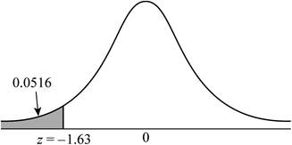
The z-score less than or equal to –1.63 represents the proportion of observations to the left of −1.63.

Use Table A: Standard normal cumulative proportions to find the area to the left of –1.63.

Procedure:

• Locate –1.6 in the left column of the table.
• Obtain the value in the corresponding row below 0.03.

That is, $P\left(z<-1.63\right)=0.0516$

Thus, the proportion of observations from a standard normal distribution that falls in $z\le -1.63$ is 0.0516.

Shade the region to the left of $z=-1.63$ as shown in Figure (1).

Figure (1)

The shaded region represents the proportion of observations less than or equal to –1.63.

(b)

To determine

To obtain: The proportion of observations from a standard normal distribution that falls in $z\ge -1.63$.

To sketch: The standard normal curve for $z\ge -1.63$.

Answer to Problem 3.28E

The proportion of observations from a standard normal distribution that falls in $z\ge -1.63$ is 0.9484.

The standard normal curve for $z\ge -1.63$ is

Explanation of Solution

Calculation:

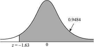
The z-score greater than or equal to –1.63 represents the proportion of observations to the right of −1.63. But, Table A: Standard normal cumulative proportions apply only for the cumulative areas to the left.

Use Table A: Standard normal cumulative proportions to find the area to the left of –1.63.

Procedure:

• Locate –1.6 in the left column of the table.
• Obtain the value in the corresponding row below 0.03.

That is, $P\left(z<-1.63\right)=0.0516$

The area to the right of –1.63 is,

$\begin{array}{c}P\left(z>-1.63\right)=1-P\left(z<-1.63\right)\\ =1-0.0516\\ =0.9484\end{array}$

Thus, the proportion of observations from a standard normal distribution that falls in $z\ge -1.63$ is 0.9484.

Shade the region to the left of $z=-1.63$ as shown in Figure (2).

Figure (2)

The shaded region in Figure (2) represents the proportion of observations greater than or equal to –1.63.

(c)

To determine

To obtain: The proportion of observations from a standard normal distribution that falls in $z>0.92$.

To sketch: The standard normal curve for $z>0.92$.

Answer to Problem 3.28E

The proportion of observations from a standard normal distribution that falls in $z>0.92$ is 0.1788.

The standard normal curve for $z>0.92$ is

Explanation of Solution

Calculation:

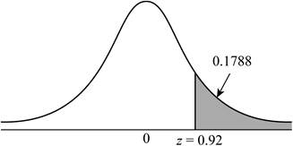
The z-score greater than 0.92 represents the proportion of observations to the right of 0.92. But, Table A: Standard normal cumulative proportions apply only for the cumulative areas to the left.

Use Table A: Standard normal cumulative proportions to find the area to the left of 0.92.

Procedure:

• Locate 0.9 in the left column of the table.
• Obtain the value in the corresponding row below 0.02.

That is, $P\left(z<0.92\right)=0.8212$

The area to the right of 0.92 is,

$\begin{array}{c}P\left(z>0.92\right)=1-P\left(z<0.92\right)\\ =1-0.8212\\ =0.1788\end{array}$

Thus, the proportion of observations from a standard normal distribution that falls in $z>0.92$ is 0.1788.

Shade the region to the left of $z>0.92$ as shown in Figure (3).

Figure (3)

The shaded region represents the proportion of observations greater than or equal to 0.92.

d)

To determine

To obtain: The proportion of observations from a standard normal distribution that falls in $-1.63<z<0.92$.

To sketch: The standard normal curve for $-1.63<z<0.92$.

Answer to Problem 3.28E

The proportion of observations from a standard normal distribution that falls in $-1.63<z<0.92$ is 0.7696.

The standard normal curve for $-1.63<z<0.92$ is

Explanation of Solution

Calculation:

The z-score between –1.63 and 0.92 represents the proportion of observations to the right of –1.63 and to the left of 0.92.

Use Table A: Standard normal cumulative proportions to find the areas.

Procedure:

For z at –1.63,

• Locate –1.6 in the left column of the table.
• Obtain the value in the corresponding row below 0.03.

That is, $P\left(z<-1.63\right)=0.0516$

For z at 0.92,

• Locate 0.9 in the left column of the table.
• Obtain the value in the corresponding row below 0.02.

That is, $P\left(z<0.92\right)=0.8212$

Hence, the difference between the areas to the left of –0.42 and the left of 2.12 is,

$\begin{array}{c}P\left(-1.63<z<0.92\right)=P\left(z<0.92\right)-P\left(z<-1.63\right)\\ =0.8212-0.0516\\ =0.7696\end{array}$

Thus, the proportion of observations from a standard Normal distribution that takes values between –1.63 and 0.92 is 0.7696.

Shade the region to the right of $z=-1.63$ to the left of $z=0.92$ as shown in Figure (4).

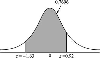
Figure (4)

The shaded region represents the proportion of observations between –1.63 and 0.92