
Videos
The paper “Lessons from Pacemaker Implantations” (Journal of the American Medical Association [1965]: 231–232) gave the results of a study that followed 89 heart patients who had received electronic pacemakers. The time (in months) to the first electrical malfunction of the pacemaker was recorded:
![Chapter 3, Problem 12CRE, The paper Lessons from Pacemaker Implantations (Journal of the American Medical Association [1965]:](https://content.bartleby.com/tbms-images/9781337793612/Chapter-3/images/93612-3-12cre-question-digital_image_001.png)
- a. Summarize these data in the form of a frequency distribution, using class intervals of 0 to <6, 6 to <12, and so on.
- b. Calculate the relative frequencies and cumulative relative frequencies for each class interval of the frequency distribution of Part (a).
- c. Show how the relative frequency for the class interval 12 to <18 could be obtained from the cumulative relative frequencies.
- d. Use the cumulative relative frequencies to give approximate answers to the following:
- i. What proportion of those who participated in the study had pacemakers that did not malfunction within the first year?
- ii. If the pacemaker must be replaced as soon as the first electrical malfunction occurs, approximately what proportion required replacement between 1 and 2 years after implantation?
- e. Construct a cumulative relative frequency plot, and use it to answer the following questions.
- i. What is the approximate time at which 50% of the pacemakers had failed?
- ii. What is the approximate time at which only 10% of the pacemakers initially implanted were still
functioning ?
a.
Construct the frequency distribution for the given data.
Answer to Problem 12CRE
The frequency distribution is given below.
| Class interval | Frequency |
| 0-<6 | 2 |
| 6-<12 | 10 |
| 12-<18 | 21 |
| 18-<24 | 28 |
| 24-<30 | 22 |
| 30-<36 | 6 |
Explanation of Solution
Calculation:
The data represents the time to the first electrical malfunction of the pacemaker for 89 heart patients.
Software procedure:
Frequency distribution:
The number of values lying in the particular interval or the number of times each value repeats is the frequency of that particular class interval or event.
The frequencies are calculated by using the tally mark. Here, the number of times each activity repeats is the frequency of that particular physical activity.
Here, the number of values time under the specified interval is the frequency of that particular class interval of time.
Here, the number of values in between the class interval 0-<6 is 2.
Therefore, the frequency of the class interval 0-<6 is 2.
Similarly, the frequencies of all the remaining class intervals are as follows:
| Class interval | Tally | Frequency |
| 0-<6 | 2 | |
| 6-<12 | 10 | |
| 12-<18 | 21 | |
| 18-<24 | 28 | |
| 24-<30 | 22 | |
| 30-<36 | 6 | |
| Total | 89 |
b.
Construct the relative frequency distribution for the given data.
Construct the cumulative relative frequency distribution for the given data.
Answer to Problem 12CRE
The relative frequency distribution and cumulative relative frequency distribution are given below.
| Class interval | Relative frequency | Cumulative relative frequency |
| 0-<6 | 0.02247 | 0.02247 |
| 6-<12 | 0.11236 | 0.13483 |
| 12-<18 | 0.23596 | 0.37079 |
| 18-<24 | 0.31461 | 0.6854 |
| 24-<30 | 0.24719 | 0.39259 |
| 30-<36 | 0.06742 | 1 |
Explanation of Solution
Calculation:
The general formula to obtain the relative frequency is given below:
Substitute the frequency of the class interval 0-<6 as “2” and the total frequency as “89” in relative frequency.
Similarly, relative frequencies for the remaining class intervals are obtained below:
| Class interval | Frequency | Relative frequency |
| 0-<6 | 2 | |
| 6-<12 | 10 | |
| 12-<18 | 21 | |
| 18-<24 | 28 | |
| 24-<30 | 22 | |
| 30-<36 | 6 |
Cumulative relative frequency:
Cumulative relative frequency is the sum of relative frequencies of all the previous events which are arranged in an order from smallest to largest value.
The general formula to obtain cumulative frequency using frequency distribution is,
From the relative frequencies, the cumulative relative frequencies are obtained as follows:
| Class interval | Relative frequency | Cumulative relative frequency |
| 0-<6 | 0.02247 | |
| 6-<12 | 0.11236 | |
| 12-<18 | 0.23596 | |
| 18-<24 | 0.31461 | |
| 24-<30 | 0.24719 | |
| 30-<36 | 0.06742 |
c.
Obtain the relative frequency for the class interval 12-18 using the cumulative frequency distribution.
Answer to Problem 12CRE
The relative frequency for the class interval 12-18 using the cumulative frequency distribution is 0.23596.
Explanation of Solution
Calculation:
The general formula to obtain cumulative frequency using frequency distribution is given below:
Relative frequency of a present event is obtained using the formula given below:
From the cumulative relative frequency distribution, relative frequency distribution is obtained as given below:
Thus, the relative frequency for the class interval 12-18 using the cumulative frequency distribution is 0.23596.
d.
(i). Find the approximate proportion of heart patients who had pacemakers that did not malfunction within the first year.
(ii) Find the approximate proportion of heart patients who required replacement between 1 and 2 years after implantation.
Answer to Problem 12CRE
(i) The approximate proportion of heart patients who had pacemakers that did not malfunction within the first year is 0.86517.
(ii) The approximate proportion of heart patients who required replacement between 1 and 2 years after implantation is 0.55057.
Explanation of Solution
Calculation:
The general formula for the relative frequency or proportion is,
(i). Approximate proportion of heart patients who had pacemakers that did not malfunction within the first year:
The Objective is to find the cumulative relative frequency of heart patients who had pacemakers that did not malfunction within the first year.
The cumulative relative frequency of heart patients who had pacemakers that malfunction within the first year is 0.13483.
That is, the proportion of heart patients who had pacemakers that malfunction within the first year is 0.13483.
Hence, the cumulative relative frequency of heart patients who had pacemakers that did not malfunction within the first year is obtained as given below:
Thus, the approximate proportion of heart patients who had pacemakers that did not malfunction within the first year is 0.86517.
(ii). Approximate proportion of heart patients who required replacement between 1 and 2 years after implantation:
The Objective is to find the relative frequency of heart patients required replacement between 1 and 2 years after implantation.
The relative frequency of heart patients required replacement between 1 and 2 years after implantation is obtained as given below:
Thus, the approximate proportion of heart patients who required replacement between 1 and 2 years after implantation is 0.55057.
e.
Plot the cumulative frequency distribution for the given data.
(i) Find the approximate time at which 50% of the pacemakers had failed.
(ii) Find the approximate time at which only 10% of the initially implanted pacemakers are functioning.
Answer to Problem 12CRE
Cumulative distribution plot is given below:
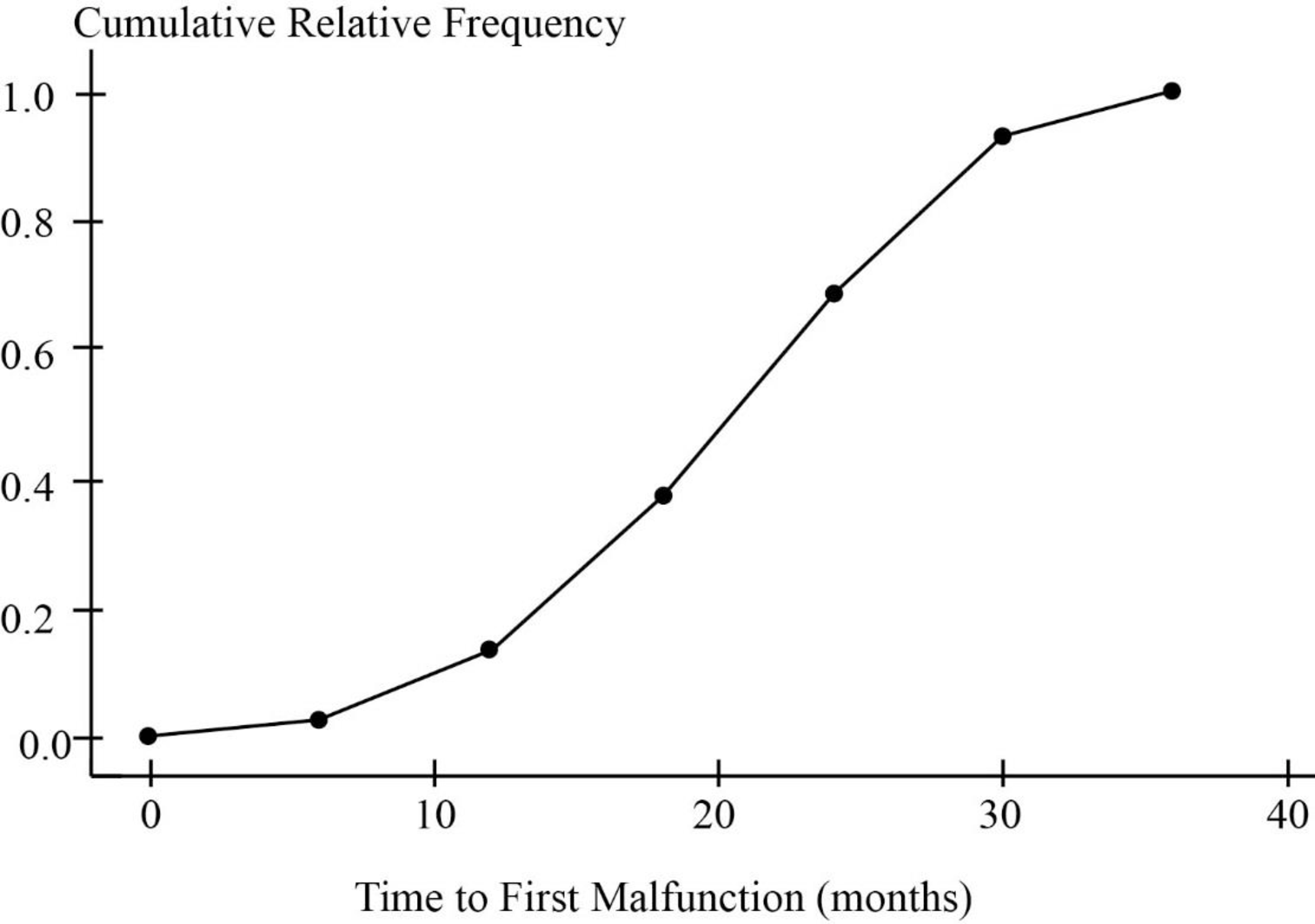
(i) The time at which 50% of the pacemakers had failed will be in between 18-<24 months.
(ii) The approximate time at which only 10% of the initially implanted pacemakers are functioning will be in between 24-<30 months.
Explanation of Solution
Calculation:
The cumulative relative frequency histogram is plotted for the given data.
Procedure to plot cumulative distribution plot:
Step by step procedure to draw the cumulative distribution plot is given below.
- Draw a horizontal axis and a vertical axis.
- The horizontal axis represents the cumulative frequencies.
- The vertical axis represents the “Time to first malfunction in months”.
- Plot each of the 6 cumulative frequencies corresponding to the time to first malfunction in months.
- Connect all the 6 plotted points of cumulative frequencies with a line.
The general formula for the relative frequency or proportion is,
(i). Approximate time at which 50% of the pacemakers had failed:
The Objective is to find the time at which 50% of the pacemakers had failed.
From the cumulative relative frequency distribution, 0.6854 corresponds to the interval 18-<24 months.
The cumulative relative frequency of 0.5 is less than the cumulative relative frequency of 0.6854.
Thus, the time at which 50% of the pacemakers had failed will be in between 18-<24 months.
(ii). Approximate time at which only 10% of the initially implanted pacemakers are functioning:
The Objective is to find the time only 10% of the initially implanted pacemakers are functioning.
In other words it can be said that, the time at which 90% of the pacemakers had failed.
From the cumulative relative frequency distribution, 0.93259 corresponds to the interval 24-<30 months.
The cumulative relative frequency of 0.9 is less than the cumulative relative frequency of 0.93259.
Thus, the time at which only 10% of the initially implanted pacemakers are functioning will be in between 24-<30 months.
Want to see more full solutions like this?
Chapter 3 Solutions
Bundle: Introduction to Statistics and Data Analysis, 5th + WebAssign Printed Access Card: Peck/Olsen/Devore. 5th Edition, Single-Term
Additional Math Textbook Solutions
Pathways To Math Literacy (looseleaf)
College Algebra (Collegiate Math)
Elementary and Intermediate Algebra: Concepts and Applications (7th Edition)
Precalculus
Elementary Statistics ( 3rd International Edition ) Isbn:9781260092561
APPLIED STAT.IN BUS.+ECONOMICS


- Examine the Variables: Carefully review and note the names of all variables in the dataset. Examples of these variables include: Mileage (mpg) Number of Cylinders (cyl) Displacement (disp) Horsepower (hp) Research: Google to understand these variables. Statistical Analysis: Select mpg variable, and perform the following statistical tests. Once you are done with these tests using mpg variable, repeat the same with hp Mean Median First Quartile (Q1) Second Quartile (Q2) Third Quartile (Q3) Fourth Quartile (Q4) 10th Percentile 70th Percentile Skewness Kurtosis Document Your Results: In RStudio: Before running each statistical test, provide a heading in the format shown at the bottom. “# Mean of mileage – Your name’s command” In Microsoft Word: Once you've completed all tests, take a screenshot of your results in RStudio and paste it into a Microsoft Word document. Make sure that snapshots are very clear. You will need multiple snapshots. Also transfer these results to the…arrow_forwardExamine the Variables: Carefully review and note the names of all variables in the dataset. Examples of these variables include: Mileage (mpg) Number of Cylinders (cyl) Displacement (disp) Horsepower (hp) Research: Google to understand these variables. Statistical Analysis: Select mpg variable, and perform the following statistical tests. Once you are done with these tests using mpg variable, repeat the same with hp Mean Median First Quartile (Q1) Second Quartile (Q2) Third Quartile (Q3) Fourth Quartile (Q4) 10th Percentile 70th Percentile Skewness Kurtosis Document Your Results: In RStudio: Before running each statistical test, provide a heading in the format shown at the bottom. “# Mean of mileage – Your name’s command” In Microsoft Word: Once you've completed all tests, take a screenshot of your results in RStudio and paste it into a Microsoft Word document. Make sure that snapshots are very clear. You will need multiple snapshots. Also transfer these results to the…arrow_forwardExamine the Variables: Carefully review and note the names of all variables in the dataset. Examples of these variables include: Mileage (mpg) Number of Cylinders (cyl) Displacement (disp) Horsepower (hp) Research: Google to understand these variables. Statistical Analysis: Select mpg variable, and perform the following statistical tests. Once you are done with these tests using mpg variable, repeat the same with hp Mean Median First Quartile (Q1) Second Quartile (Q2) Third Quartile (Q3) Fourth Quartile (Q4) 10th Percentile 70th Percentile Skewness Kurtosis Document Your Results: In RStudio: Before running each statistical test, provide a heading in the format shown at the bottom. “# Mean of mileage – Your name’s command” In Microsoft Word: Once you've completed all tests, take a screenshot of your results in RStudio and paste it into a Microsoft Word document. Make sure that snapshots are very clear. You will need multiple snapshots. Also transfer these results to the…arrow_forward
- 2 (VaR and ES) Suppose X1 are independent. Prove that ~ Unif[-0.5, 0.5] and X2 VaRa (X1X2) < VaRa(X1) + VaRa (X2). ~ Unif[-0.5, 0.5]arrow_forward8 (Correlation and Diversification) Assume we have two stocks, A and B, show that a particular combination of the two stocks produce a risk-free portfolio when the correlation between the return of A and B is -1.arrow_forward9 (Portfolio allocation) Suppose R₁ and R2 are returns of 2 assets and with expected return and variance respectively r₁ and 72 and variance-covariance σ2, 0%½ and σ12. Find −∞ ≤ w ≤ ∞ such that the portfolio wR₁ + (1 - w) R₂ has the smallest risk.arrow_forward
- 7 (Multivariate random variable) Suppose X, €1, €2, €3 are IID N(0, 1) and Y2 Y₁ = 0.2 0.8X + €1, Y₂ = 0.3 +0.7X+ €2, Y3 = 0.2 + 0.9X + €3. = (In models like this, X is called the common factors of Y₁, Y₂, Y3.) Y = (Y1, Y2, Y3). (a) Find E(Y) and cov(Y). (b) What can you observe from cov(Y). Writearrow_forward1 (VaR and ES) Suppose X ~ f(x) with 1+x, if 0> x > −1 f(x) = 1−x if 1 x > 0 Find VaRo.05 (X) and ES0.05 (X).arrow_forwardJoy is making Christmas gifts. She has 6 1/12 feet of yarn and will need 4 1/4 to complete our project. How much yarn will she have left over compute this solution in two different ways arrow_forward
- Solve for X. Explain each step. 2^2x • 2^-4=8arrow_forwardOne hundred people were surveyed, and one question pertained to their educational background. The results of this question and their genders are given in the following table. Female (F) Male (F′) Total College degree (D) 30 20 50 No college degree (D′) 30 20 50 Total 60 40 100 If a person is selected at random from those surveyed, find the probability of each of the following events.1. The person is female or has a college degree. Answer: equation editor Equation Editor 2. The person is male or does not have a college degree. Answer: equation editor Equation Editor 3. The person is female or does not have a college degree.arrow_forwardneed help with part barrow_forward
 Glencoe Algebra 1, Student Edition, 9780079039897...AlgebraISBN:9780079039897Author:CarterPublisher:McGraw Hill
 Functions and Change: A Modeling Approach to Coll...AlgebraISBN:9781337111348Author:Bruce Crauder, Benny Evans, Alan NoellPublisher:Cengage Learning
 Holt Mcdougal Larson Pre-algebra: Student Edition...AlgebraISBN:9780547587776Author:HOLT MCDOUGALPublisher:HOLT MCDOUGAL